zkSecurity
Audit Report

Audit of Midnight Halo2 Fork

Midnight • March 3rd, 2025

Introduction

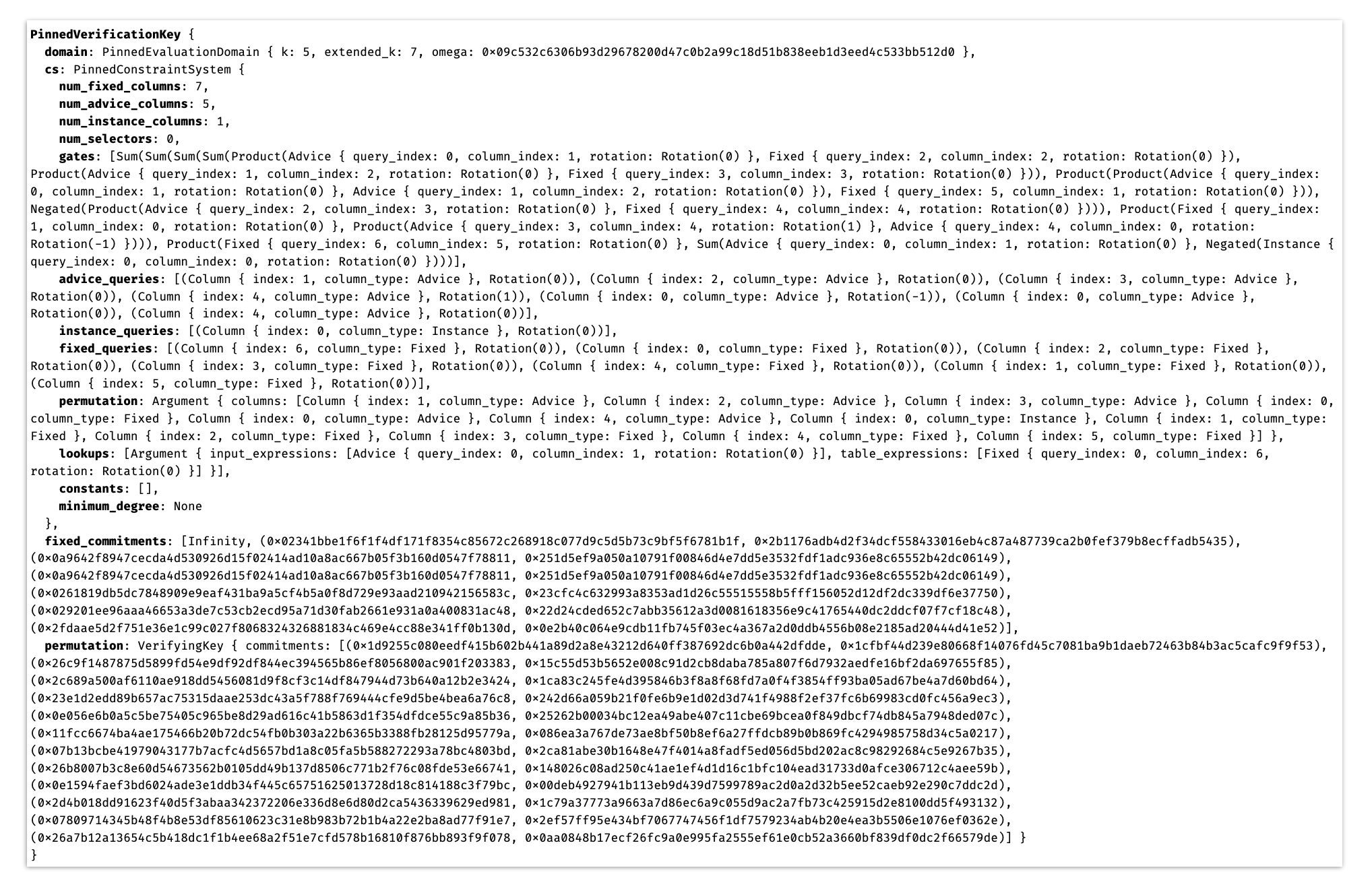
On March 3rd, 2025, zkSecurity was tasked to audit the Midnight Halo2 fork. The specific code to review was shared via GitHub as a public repository (https://github.com/midnightntwrk/halo2 at commit 417f29a5c0ede5d98825b95c8e8e9a1532ec177c). The audit was conducted between March 3rd, 2025 and March 28th, 2025 by two consultants. The audit focused on the correctness and security of the generalized Plonk implementation as well as circuit framework in the Midnight fork.

The code was found to be clean and well organized. Several observations and findings have been reported to the Midnight team, which are detailed in the following sections.

Scope

The scope of this audit is the whole Midnight Halo2 framework, which is forked from PSE Halo2. The differences between the main Halo2 forks are described below.

Halo2

Halo2 is a zero-knowledge proof system that implements the ideas developed by the team behind the Electric Coin Company’s (ECC) Zcash. The current open source system is a result of various iterations of the system, starting with efforts in 2019 (original Halo and its related publication). The resulting current Halo2 is a zk-SNARK system based on PLONK but several enhancements to allow for more general, custom gates and lookups. It also allows recursive proofs and does not need a per-circuit trusted setup, but instead relies on a one-time universal setup. It is a popular proof system that is used beyond Zcash: at the time of writing this report (March 2025), it has over 500 forks and over 700 projects use it. It has seen over 30 contributors and closed over 400 pull requests. Halo2 powers the Zcash Orchard protocol since 2022.

The PSE fork

The most popular Halo2 fork is the one from the PSE (Privacy and Scaling Explorations) group at the Ethereum Foundation. This fork is tailored for Ethereum-oriented use cases involving on-chain verification. Therefore, it focuses on the BN254 curve and KZG commitments, instead of the original “Halo” style using Pasta curves. This is because BN254 offers a convenient precompile on Ethereum mainnet, making on-chain verification cheaper. KZG commitments over BN254 are standard in many Ethereum-based ZK rollups. This fork also implements a re-architecture of the original codebase, splitting frontend and backend. PSE merges many upstream changes from the ECC code, but diverges on some features, for instance those related to EVM compatibility.

The Midnight fork

In this report we audit the Midnight fork of the PSE fork. The main differences with respect to the PSE fork are as follows. First, a number of unused features were removed, such as compressed selectors, IPA and the use of SHPLONK for proof aggregation. Moreover the interfaces of KZG and polynomial commitment scheme were rewritten. Finally, a configuration feature was added to allow for truncated challenges, used mainly during KZG. Such a truncation aims at improving efficiency while preserving security.

Overview

Halo2 Frontend API Overview

Two key interfaces at the front-end, Circuit::configure and Circuit::synthesize, give developers flexibility in composing circuits while encapsulating most of the low-level complexity.

Create a gate constraint

Circuit::configure is used to define gate constraints. It provides access to the ConstraintSystem API, through which developers specify constraint expressions. Below is an example of defining a multiplication gate constraint:

fn configure(
    meta: &mut ConstraintSystem<F>
) -> <Self as Chip<F>>::Config {
    // We create the two advice columns that FieldChip uses for I/O.
    let advice = [meta.advice_column(), meta.advice_column()];

    // We also need an instance column to store public inputs.
    let instance = meta.instance_column();

    // Create a fixed column to load constants.
    let constant = meta.fixed_column();

    meta.enable_equality(instance);
    meta.enable_constant(constant);
    for column in &advice {
        meta.enable_equality(*column);
    }
    let s_mul = meta.selector();

    // Define our multiplication gate
    meta.create_gate("mul", |meta| {
        let lhs = meta.query_advice(advice[0], Rotation::cur());
        let rhs = meta.query_advice(advice[1], Rotation::cur());
        let out = meta.query_advice(advice[0], Rotation::next());
        let s_mul = meta.query_selector(s_mul);

        vec![s_mul * (lhs * rhs - out)]
    });

    FieldConfig {
        advice,
        instance,
        s_mul,
    }
}

Developers can create new columns (advice, instance, and fixed). Advice columns store runtime witness values, instance columns store public inputs, and fixed columns hold compile-time constants. Each of these columns may be “equality-enabled” to participate in copy constraints.

enable_equality/enable_constant To avoid unnecessary overhead in the permutation argument, developers must manually enable equality for columns that will be involved in copy constraints or equality checks. Notice that the constant column is not directly constrained in this gate, but we enable equality on it to allow constraining a cell to a constant value later.

Selector A selector expression is a virtual column, which is not materialized like the columns until key generation phase. In vanilla Plonk, there are simple and complex selectors. Simple selectors only allow to be applied to entire gate constraints (e.g., q * (A * B - C)), while complex selectors can appear inside expressions (e.g., A * B - q * C).

In this midnight fork, the simple selector is unnecessary, as it does not use selector-combining optimizations. Ultimately, the selector expression is turned into a fixed-column value during key generation.

create_gate ConstraintSystem::create_gate defines a gate constraint. In the snippet above, lhs, rhs, and out are queries referencing specific columns and rotations, while s_mul is the selector expression that eventually becomes a fixed column. The multiplication gate is enforced by the polynomial expression:

s_mul * (lhs * rhs - out)

The expression’s internal data structure looks like:

[
    Product(
        Selector(
            Selector(0, true)
        ), 
        Sum(
            Product(
                Advice { query_index: 0, column_index: 0, rotation: Rotation(0) }, 
                Advice { query_index: 1, column_index: 1, rotation: Rotation(0) }
            ), 
            Negated(Advice { query_index: 2, column_index: 0, rotation: Rotation(1) })
        )
    )
]

In this case, Advice and Selector are the lowest level expressions, while the others like Product, Sum and Negated are composable expressions. By providing the evaluations for the lowest level expressions, a composed expression can be evaluated recursively.

During proving, this structure represents a gate constraint polynomial in the vanishing polynomial evaluation. The query_index indicates how the verifier loads the corresponding cell evaluation from the transcript, as in:

// load evals from transcript
let advice_evals = (0..num_proofs)
    .map(|_| -> Result<Vec<_>, _> { read_n(transcript, vk.cs.advice_queries.len()) })
    .collect::<Result<Vec<_>, _>>()?;

let fixed_evals = read_n(transcript, vk.cs.fixed_queries.len())?;

// load an eval based on query index embedded in expression
gate.polynomials().iter().map(move |poly| {
    poly.evaluate(
        &|query| fixed_evals[query.index.unwrap()],
        &|query| advice_evals[query.index.unwrap()],

..TRUNCATED

Synthesize circuit

Circuit::synthesize is responsible for circuit construction. It provides the Layouter API, which lets developers build regions and wire cells. Below is an example of synthesizing the multiplication gate:

fn mul(
    &self,
    mut layouter: impl Layouter<F>,
    a: AssignedCell,
    b: AssignedCell,
) -> Result<AssignedCell, Error> {
    let config = self.config();

    layouter.assign_region(
        || "mul",
        |mut region: Region<'_, F>| {
            config.s_mul.enable(&mut region, 0)?;

            a.0.copy_advice(|| "lhs", &mut region, config.advice[0], 0)?;
            b.0.copy_advice(|| "rhs", &mut region, config.advice[1], 0)?;

            let value = a.0.value().copied() * b.0.value();

            region
                .assign_advice(|| "lhs * rhs", config.advice[0], 1, || value)
                .map(Number)
        },
    )
}

A region is a consecutive set of rows in which constraints can be applied. The assign_region method specifies the logic for that region, including copy constraints, gate constraints and witness generation. Selectors are enabled by referencing a region and a specific row in that region.

Copy Constraint The copy_advice method can wire cells from anywhere in the circuit, include the cells from the other regions. Internally, it updates the permutation mapping using the cells’ column indices and row offsets:

fn constrain_equal(&mut self, left: Cell, right: Cell) -> Result<(), Error> {
    self.plan.cs.copy(
        left.column,
        *self.plan.regions[*left.region_index] + left.row_offset,
        right.column,
        *self.plan.regions[*right.region_index] + right.row_offset,
    )?;

    Ok(())
}

Here, the actual row offset is calculated from the region index stored within each cell.

Witness Generation The value method returns the cell’s value for witness generation. In practice, witness generation and circuit construction are separate. The Assignment trait enables this separation:

During proving, WitnessCollection implements Assignment to gather witness values.
Assembly handles fixed values (constants, permutation mappings, static lookup tables) for key generation, where these values must be committed.

Convert to Fixed Columns

Constraint Constants The earlier configure example does not explicitly use the constant column inside create_gate, but it may still be necessary. Whenever a cell must be constrained to a constant value, that constant is first assigned to a constant (fixed) column, then a copy constraint is applied from the constant cell to the advice cell. The front-end provides assign_advice_from_constant for this:

fn assign_advice_from_constant<'v>(
    &'v mut self,
    annotation: &'v (dyn Fn() -> String + 'v),
    column: Column<Advice>,
    offset: usize,
    constant: Rational<F>,
) -> Result<Cell, Error> {
    let advice =
        self.assign_advice(annotation, column, offset, &mut || Value::known(constant))?;
    self.constrain_constant(advice, constant)?;

    Ok(advice)
}

Behind the scenes, the tuple (cell, constant) recorded by constrain_constant is used to create a copy constraint from the constant cell to the advice cell via ConstraintSystem::assign_fixed and ConstraintSystem::copy:

for (constant, advice) in constants_to_assign {
    self.cs.assign_fixed(
        || format!("Constant({:?})", constant.evaluate()),
        constants_column,
        *next_constant_row,
        || Value::known(constant),
    )?;
    self.cs.copy(
        constants_column.into(),
        *next_constant_row,
        advice.column,
        *self.regions[*advice.region_index] + advice.row_offset,
    )?;
    *next_constant_row += 1;
}

Materialize Selectors Each virtual selector must be converted to a fixed column before computing commitments during key generation. The replace_selectors_with_fixed method accomplishes this:

pub fn directly_convert_selectors_to_fixed(
    mut self,
    selectors: Vec<Vec<bool>>,
) -> (Self, Vec<Vec<F>>) {
    // The number of provided selector assignments must be the number we
    // counted for this constraint system.
    assert_eq!(selectors.len(), self.num_selectors);

    let (polys, selector_replacements): (Vec<_>, Vec<_>) = selectors
        .into_iter()
        .map(|selector| {
            let poly = selector
                .iter()
                .map(|b| if *b { F::ONE } else { F::ZERO })
                .collect::<Vec<_>>();
            let column = self.fixed_column();
            let rotation = Rotation::cur();
            let expr = Expression::Fixed(FixedQuery {
                index: Some(self.query_fixed_index(column, rotation)),
                column_index: column.index,
                rotation,
            });
            (poly, expr)
        })
        .unzip();

    self.replace_selectors_with_fixed(&selector_replacements);
    self.num_selectors = 0;

    (self, polys)
}

In the process, the selector expressions are converted to fixed column expressions, and the number of selectors is reset to zero. After this, the commitments to the selectors can be computed directly from the fixed column values.

Frontend Layouter, RegionLayouter, and Assignment Overview

Given a circuit, Halo2 will call the Circuit::synthesize function to layout the circuit and assign the cells during key generation and proving time. Halo2 uses three key traits from top-down to manage the layout and assignment: Layouter, RegionLayouter, and Assignment. To assign a cell in the circuit, Halo2 typically calls these traits top-down:

–> Circuit.synthesize
–-> Layouter.assign_region
–--> RegionLayouter.assign_advice
–---> Assignment.assign_advice

Layouter Trait is responsible for managing and laying out all regions. You can imagine each region to be a rectangle with different width and height. The layouter needs to arrange these regions (with no overlap) in a big table. For efficiency reasons, the big table should have as few rows as possible.

NamespacedLayouter in src/circuit/mod.rs: this layouter is used for debugging. It keeps the current namespace string and wraps other layouters.
SingleChipLayouter in src/circuit/floor_planner/single_pass.rs: this is the simplest layouter strategy. It just aligns regions by the given order. The current region is placed at the first available row.
V1Pass in src/circuit/floor_planner/v1.rs: it lays out the region using a greedy strategy. It sorts the regions by area (num_advice_column * num_row) in descending order. It places regions from largest to smallest. When placing the current region, it will try to find if there is a gap (that is large enough to fit the current region) among previous regions. If so, it places the current region in the gap; otherwise, it places the region in the first available row.

RegionLayouter Trait is for tracking states inside one region.

RegionShape in src/circuit/layouter.rs: it tracks the number of rows in the region, considering only the row count and ignoring the assigned values.
SingleChipLayouterRegion in src/circuit/floor_planner/single_pass.rs: it’s the region layouter for SimpleFloorPlanner layouter.
V1Region for src/circuit/floor_planner/v1.rs: it’s the region layouter for V1 layouter.

The main difference between SingleChipLayouterRegion and V1Region is how they handle constants.

Assignment Trait is for tracking the assignment of cells in Advice column and Fixed column

Assembly in src/plonk/keygen.rs: for tracking fixed column values (including selector) and the copy constraint (for permutation). The assignment in advice column is ignored. This is used to generate verifying key, including fixed column commitment and permutation commitment.
WitnessCollection in src/plonk/prover.rs: for the prover to collect witness (i.e., the value in the advice columns). This is used in proving time.

Key Generation Overview

Key generation is the process of generating the proving key and the verifying key. The verifying key is constructed from the circuit and contains information about the circuit as well as commitments to public columns. The proving key contains the verifying key along with auxiliary polynomials necessary for creating zero-knowledge proofs. Simply put, key generation converts the representation of the circuit from a large table to a set of polynomials evaluated in the extended domain, which can then be used in the backend to either create or verify a proof.

Verifying Key

/// This is a verifying key which allows for the verification of proofs for a
/// particular circuit.
#[derive(Clone, Debug)]
pub struct VerifyingKey<F: PrimeField, CS: PolynomialCommitmentScheme<F>> {
    domain: EvaluationDomain<F>,
    fixed_commitments: Vec<CS::Commitment>,
    permutation: permutation::VerifyingKey<F, CS>,
    cs: ConstraintSystem<F>,
    cs_degree: usize,
    transcript_repr: F,
}

/// NOTE: permutation::VerifyingKey
/// The verifying key for a single permutation argument.
#[derive(Clone, Debug)]
pub struct VerifyingKey<F: PrimeField, CS: PolynomialCommitmentScheme<F>> {
    commitments: Vec<CS::Commitment>,
}

The first step in constructing a verifying key is to set a value k, where 2^k corresponds to the number of rows in the final table. This value can be set automatically by calling keygen_vk with a ConcreteCircuit instance and PolynomialCommitmentScheme::Parameters, or the caller can specify a value using keygen_vk_with_k. Note that 2^k should be large enough to accommodate the rows required by the circuit as well as the blinding factors.

The second step is to synthesize the circuit. This is done by calling ConcreteCircuit::FloorPlanner::synthesize, which, by default, invokes the synthesize method on the circuit. As detailed in our overview of the Frontend APIs, the synthesize method constructs the circuit by building regions and wire constraints. At this point, if the specified 2^k value is not large enough to accommodate the circuit, a NotEnoughRowsAvailable error will be thrown.

The next step is to merge the selector polynomials with the fixed polynomials by converting the boolean values of the selectors to field elements (0 or 1) and appending them to the fixed polynomials. Each of these polynomials is then committed using the commit_lagrange method of the polynomial commitment scheme, which performs Multi-Scalar Multiplication (MSM) with the Structured Reference String (SRS) of the KZG commitment scheme.

Finally, we build the verifying key for the permutation argument, which consists of commitments to the permutation polynomials. As outlined in the Halo2 book, the cells of the permutation columns are populated by permuted indices, where the index is defined by $δ^{j} \cdot ω^{i}$ for the i-th row and the j-th column.

Proving Key

/// This is a proving key which allows for the creation of proofs for a
/// particular circuit.
#[derive(Clone, Debug)]
pub struct ProvingKey<F: PrimeField, CS: PolynomialCommitmentScheme<F>> {
    vk: VerifyingKey<F, CS>,
    l0: Polynomial<F, ExtendedLagrangeCoeff>,
    l_last: Polynomial<F, ExtendedLagrangeCoeff>,
    l_active_row: Polynomial<F, ExtendedLagrangeCoeff>,
    fixed_values: Vec<Polynomial<F, LagrangeCoeff>>,
    fixed_polys: Vec<Polynomial<F, Coeff>>,
    fixed_cosets: Vec<Polynomial<F, ExtendedLagrangeCoeff>>,
    permutation: permutation::ProvingKey<F>,
    ev: Evaluator<F>,
}

/// NOTE: permutation::ProvingKey
/// The proving key for a single permutation argument.
#[derive(Clone, Debug)]
pub(crate) struct ProvingKey<F: PrimeField> {
    permutations: Vec<Polynomial<F, LagrangeCoeff>>,
    polys: Vec<Polynomial<F, Coeff>>,
    pub(super) cosets: Vec<Polynomial<F, ExtendedLagrangeCoeff>>,
}

The implementation of proving key generation is similar to verifying key generation, with some key differences:

The proving key generation takes a VerifyingKey as an argument, meaning it is not possible to set a custom k value.
Instead of creating commitments to the fixed and permutation polynomials, the proving key generation interpolates them to obtain their coefficients and evaluates them in the extended domain.
The proving key generation computes selector polynomials for the blinding factors, namely l_0(X), l_last(X), and l_active_row(X). See this section for more details.
The proving key also creates an Evaluator for the circuit, which generates an optimized data structure for evaluating the circuit.

Some important notes about how the polynomials are represented in the proving key:

The polynomials are represented as Lagrange polynomial evaluations, which speeds up the computation of addition and multiplication over polynomials compared to using coefficient form.
The polynomials are “blown up” to a larger degree to account for the increased degree of the resulting polynomial from the multiplication of the selector polynomials.
The polynomials are not evaluated in the blown-up multiplicative group but rather in the coset of the blown-up multiplicative group. In the case of Halo2, this is achieved by evaluating the polynomials at $ζ \cdot x$ instead of $x$ , where $ζ = 3$ is a cube root of unity. Refer to this outline for more details on why this is necessary.

Proof System Overview

The proof system used in this protocol is very similar to the original Halo2 proving system. The most notable difference is that this protocol uses KZG as the polynomial commitment scheme instead of the Inner Product Argument (IPA) used in the original Halo2 protocol.

Throughout the protocol, the commitment of a polynomial $a (X)$ is denoted by $[a]_{1}$ , which represents the KZG commitment of $a (X)$ . This is computed by performing Multi-Scalar Multiplication (MSM) on the coefficients of $a (X)$ as scalars against structured group elements $G_{i} = [τ^{i}] 𝔾_{1}$ , which are generated during a trusted setup using the secret $τ$ .

At a high level, the Halo2 proof system consists of the following interactions between the prover and the verifier.

Circuit Commitments

At the start of the protocol, the prover possesses a table of cell assignments that satisfy the constraint system. This table consists of $n = 2^{k}$ rows, divided into:

Fixed columns denoted by $F_{i, j}$
Advice and instance columns denoted by $A_{i, j}$

where $A_{i, j}$ corresponds to the $i$ -th row and $j$ -th column.

Prover: Commits $a (X)$ and $f (X)$ to the verifier:

$A$ $= ([a_{0} (X)]_{1}, [a_{1} (X)]_{1}, . . ., [a_{i} (X)]_{1})$ as purported commitment of $a (X)$
$F$ $= ([f_{0} (X)]_{1}, [f_{1} (X)]_{1}, . . ., [f_{i} (X)]_{1})$ as purported commitment of $f (X)$

where $a_{i} (X)$ and $f_{i} (X)$ are Lagrange polynomials interpolating such that:

$a_{i} (ω^{j}) = A_{i, j}$
$f_{i} (ω^{j}) = F_{i, j}$

Verifier: The verifier receives $A$ and $F$ , then samples a random challenge $θ$

Prover: Given a lookup with input column polynomials $A_{i} (X)$ and table column polynomials $S_{i} (X)$ for all $i$ in $m$ rows, the prover calculate the following to compress the polynomials using $θ$ :

A_{c o m p r e s s e d} (X) = \sum_{i = 0}^{m - 1} θ^{m - 1 - i} A_{i} (X)

S_{c o m p r e s s e d} (X) = \sum_{i = 0}^{m - 1} θ^{m - 1 - i} S_{i} (X)

The prover then permutes these compressed polynomials, obtaining $A^{'} (X)$ and $S^{'} (X)$ , according to the lookup argument.

The prover commits $L$ $= ([A^{'} (X)]_{1}, [S^{'} (X)]_{1}, . . .)$ to the verifier.

Verifier: The verifier receives $L$ and samples random challenges $β$ and $γ$ .

Prover: The prover constructs $Z_{P}$ and $Z_{L}$ as equality constraint permutation polynomial and lookup permutation product polynomial respectively, according to the permutation argument and lookup argument.

Then, the prover commits these polynomials:

$Z_{P}$ $= ([Z_{P, 0} (X)]_{1}, [Z_{P, 1} (X)]_{1}, . . .)$
$Z_{L}$ $= ([Z_{L, 0} (X)]_{1}, [Z_{L, 1} (X)]_{1}, . . .)$

After all circuit commitments are committed, the protocol will perform vanishing argument to ensure the satisfiability of circuit relations.

Vanishing Argument

Vanishing argument is the protocol to demonstrate that the Halo2 circuit relations are satisfied, specifically it satisfies all the gates and custom gates, lookup arguments, and the equality constraint permutations.

Prover: The prover commit random polynomial $r (X)$ for degree $n - 1$ for blinding.

Verifier: The verifier samples a random challenge $y$ .

Prover: The prover construct the following polynomial:

h (X) = \frac{g a t e_{0} (X) + y \cdot g a t e_{1} (X) + . . . + y^{i} \cdot g a t e_{i} (X)}{t (X)}

where $g a t e_{i} (X)$ is polynomial representing the gate in the circuit (which can include polynomial $a (X)$ and $f (X)$ as well), and $t (X)$ is vanishing polynomial $(X^{n} - 1)$ . If the numerator polynomial is perfectly divisible by $t (X)$ , then the circuit relations are satisfied with high probability.

Then, the prover split the polynomial $h (X)$ into pieces of smaller-degree polynomial:

h_{0} (X) + X^{n} h_{1} (X) + . . . + X^{n (d - 1)} h_{d - 1} (X)

The prover commits $H$ $= ([h_{0} (X)]_{1}, [h_{1} (X)]_{1}, . . ., [h_{d - 1} (X)]_{1})$ to the verifier.

Verifier: Receives commitment $H$ and samples a random challenge $x$ .

Prover: The prover evaluates all polynomials that have been committed so far, using evaluation point $x$ (this includes polynomial $r (X)$ ). Then, the prover send all these evaluations to the verifier.

Verifier: The verifier receives all the evaluations and check that these evaluations satisfy the form of $h (X)$ :

\frac{g a t e_{0} (x) + y \cdot g a t e_{1} (x) + . . . + y^{i} \cdot g a t e_{i} (x)}{t (x)} = h_{0} (x) + x^{n} h_{1} (x) + . . . + x^{n (d - 1)} h_{d - 1} (x)

If the above check is satisfied, then the verifier can conclude that the circuit relations are satisfied. However, the verifier needs one remaining check that the evaluations themselves are consistent with the original commitments that have been made throughout the protocol. This check is done by the multipoint opening argument below.

Multipoint Opening Overview

Background:

At the end of Halo2 verification, the verifier has KZG commitments of multiple polynomials and wants to evaluate them at different points. The naive way is to evaluate each polynomial and each point one-by-one. That is apparently not efficient enough. We would like to evaluate them in one batch to reduce the proof size and the computation.

Let’s say given committed function $a (X)$ , $b (X)$ , $c (X)$ , and $d (X)$ . We want to evaluate $a (X)$ and $b (X)$ on point $z$ , evaluate $c (X)$ and $d (X)$ on $z$ and $ω z$ , where $ω$ denotes the root of unity of the evaluation domain. The general idea is to evaluate $a (X)$ and $b (X)$ in a batch, $c (X)$ and $d (X)$ in another batch, and verify them together.

Notations

Below are some functions defined in the protocol. We put them here just for convenient reference. $x_{1}$ , $x_{2}$ , $x_{3}$ , and $x_{4}$ are random elements sampled by the verifier. Define $q_{1} (X)$ as random linear combination of $a (X)$ and $b (X)$ , $q_{2} (X)$ as random linear combination of $c (X)$ and $d (X)$ :

\begin{matrix} q_{1} (X) : = a (X) + x_{1} b (X) \\ q_{2} (X) : = c (X) + x_{1} d (X) \end{matrix}

Define $V_{1} (X)$ as the vanishing polynomial $V_{1} (X) : = (X - z)$ . The same for $V_{2} (X) : = (X - z) (X - ω z)$ . $I_{1} (X)$ is the interpolated polynomial such that $I_{1} (z) = q_{1} (z)$ . Same, $I_{2} (X)$ is the interpolated polynomial such that $I_{2} (z) = q_{2} (z)$ and $I_{2} (ω z) = q_{2} (ω z)$ . Then we have the quotient polynomial for $q_{1}$ and $q_{2}$ :

\begin{matrix} f_{1} (X) : = \frac{q_{1} (X) - I_{1} (X)}{V_{1} (X)} \\ f_{2} (X) : = \frac{q_{2} (X) - I_{2} (X)}{V_{2} (X)} \end{matrix}

Define $f (X)$ as the random linear combination of $f_{1}$ and $f_{2}$ :

f (X) : = f_{1} (X) + x_{2} f_{2} (X)

Define $f_{f i n a l} (X)$ as the random linear combination of $f$ , $q_{1}$ and $q_{2}$ :

f_{f i n a l} (X) : = f (X) + x_{4} q_{1} (X) + x_{4}^{2} q_{2} (X)

Interaction

Prover: Send the KZG commitment of the polynomial $a_c o m$ , $b_c o m$ , $c_c o m$ and $d_c o m$ . Send the purported evaluation values $a (z)$ , $b (z)$ , $c (z)$ , $d (z)$ , $c (ω z)$ , and $d (ω z)$ .

Verifier: The verifier would like to batch $a_c o m$ and $b_c o m$ , $c_c o m$ and $d_c o m$ . It samples a random element $x_{1}$ to combine the commitment:

\begin{matrix} q_{1}_c o m : = a_c o m + x_{1} * b_c o m \\ q_{2}_c o m : = c_c o m + x_{1} * d_c o m \end{matrix}

Note that the verifier can compute the evaluation of at $q_{1} (z)$ , $q_{2} (z)$ and $q_{2} (ω z)$ : $\begin{matrix} q_{1} (z) : = a (z) + x_{1} * b (z) \\ q_{2} (z) : = c (z) + x_{1} * d (z) \\ q_{2} (ω z) : = c (ω z) + x_{1} * d (ω z) \end{matrix}$

Further, the verifier samples a random element $x_{2}$ to combine q_1 and q_2.

Prover: Compute $\begin{matrix} f (X) : = f_{1} (X) + x_{2} f_{2} (X) \\ = \frac{q_{1} (X) - I_{1} (X)}{V_{1} (X)} + x_{2} \frac{q_{2} (X) - I_{2} (X)}{V_{2} (X)} \end{matrix}$ Commit the function $f$ to $f_c o m$ .

Verifier: Receive the purported $f_c o m$ . The verifier needs to check if $f_c o m$ is correct. It would like to check the commitment at a random point. Therefore it samples $x_{3}$ and wants to check if $f (x_{3}) = = f_{1} (x_{3}) + x_{2} * f_{2} (x_{3})$

However, the Verifier cannot evaluate $f_{1} (x_{3})$ and $f_{2} (x_{3})$ on its own. Instead, it asks the prover for help.

Prover: Calculate $q_{1} (x_{3})$ and $q_{2} (x_{3})$ . Send these values to the Verifier.

Verifier: Receive the purported $q_{1} (x_{3})$ and $q_{2} (x_{3})$ . The verifier needs to check if these values are correct. Now it can compute the value $f (x_{3})$ :

\begin{matrix} f (x_{3}) : = f_{1} (x_{3}) + x_{2} * f_{2} (x_{3}) \\ = \frac{q_{1} (x_{3}) - I_{1} (x_{3})}{V_{1} (x_{3})} + x_{2} \frac{q_{2} (x_{3}) - I_{2} (x_{3})}{V_{2} (x_{3})} \end{matrix}

Now the Verifier has two things to check:

Check the value $f (x_{3})$ against the purported commitment $f_c o m$ .
Check the purported $q_{1} (x_{3})$ and $q_{2} (x_{3})$ values against the commitment $q_{1}_c o m$ and $q_{2}_c o m$ .

Again, sample a random number and batch these checks together. Sample $x_{4}$ and apply linear combinator to these checks. Combine the commitment: $f i n a l_c o m = f_c o m + x_{4} * q_{1}_c o m + x_{4}^{2} * q_{2}_c o m$ . Combine the evaluate value: $\begin{matrix} v : = f i n a l_f (x_{3}) \\ = f (x_{3}) + x_{4} * q_{1} (x_{3}) + x_{4}^{2} * q_{2} (x_{3}) \\ = (\frac{q_{1} (x_{3}) - I_{1} (x_{3})}{V_{1} (x_{3})} + x_{2} \frac{q_{2} (x_{3}) - I_{2} (x_{3})}{V_{2} (x_{3})}) + x_{4} * q_{1} (x_{3}) + x_{4}^{2} * q_{2} (x_{3}) \end{matrix}$

The last thing to do is to check $f i n a l_c o m$ against $v$ .

Prover:

Create the KZG openings $π$ that shows $f i n a l_f (x_{3}) = v$ :

h (X) : = \frac{f_{f i n a l} (X) - v}{X - x_{3}}

π : = [h (τ)]_{1}

Verifier:

Verify that $f i n a l_f (x_{3}) = v$ using $π$ . If that check passes, it means that the purported $q_{1} (x_{3})$ and $q_{2} (x_{3})$ values are consistent with $q_{1}_c o m$ and $q_{2}_c o m$ . This means that the value $f (x_{3})$ is consistent with the commitment $f_c o m$ . Then it means $f_c o m$ is indeed the commitment of the combined quotient polynomial. Finally this means that these evaluations ( $a (z)$ , $b (z)$ , $c (z)$ , $d (z)$ , $c (ω z)$ , and $d (ω z)$ ) are correct.

Blinding Overview

In this section we explain how blinding works to turn the protocol zero-knowledge.

Blinding Factors For Advice Columns

Every witness column is sent as a commitment as part of the protocol. Due to this, information leakage can happen due to two reasons:

An attacker can produce many witness values and commit to them to see if they match the committed witness (as KZG is implemented without hiding).
Each evaluation of a committed polynomial can leak information on the polynomial itself (and with enough evaluations a polynomial and the column it represents can be reconstructed).

To tackle both issues, witness columns are randomized with blinding factors. That is, some of the rows are filled with randomly generated field elements.

We know that we need at least as many blinding factors as evaluations to perfectly blind each of the prover’s witness columns.

The number of blinding factors is documented as part of the blinding_factors function which tries to account for all the evaluations in the protocol:

impl<F: Field> ConstraintSystem<F> {
    /// Compute the number of blinding factors necessary to perfectly blind
    /// each of the prover's witness polynomials.
    pub fn blinding_factors(&self) -> usize {
        // All of the prover's advice columns are evaluated at no more than
        let factors = *self.num_advice_queries.iter().max().unwrap_or(&1);
        // distinct points during gate checks.

        // - The permutation argument witness polynomials are evaluated at most 3 times.
        // - Each lookup argument has independent witness polynomials, and they are
        //   evaluated at most 2 times.
        let factors = std::cmp::max(3, factors);

        // Each polynomial is evaluated at most an additional time during
        // multiopen (at x_3 to produce q_evals):
        let factors = factors + 1;

        // h(x) is derived by the other evaluations so it does not reveal
        // anything; in fact it does not even appear in the proof.

        // h(x_3) is also not revealed; the verifier only learns a single
        // evaluation of a polynomial in x_1 which has h(x_3) and another random
        // polynomial evaluated at x_3 as coefficients -- this random polynomial
        // is "random_poly" in the vanishing argument.

        // Add an additional blinding factor as a slight defense against
        // off-by-one errors.
        factors + 1
    }

As shown above, the calculation accounts not only for the evaluations that appear as part of the constraints, but also:

An additional evaluation at $x_{3}$ is accounted which we talk about in the Multipoint Opening Overview section.
An additional blinding factor is added as a slight defense against off-by-one errors. We think this is a great idea as the slightest mistake here might lead to zero-knowledge issues.

The calculated number of blinding factors is later used in the protocol for the prover to blind each of the advice columns. In src/plonk/prover.rs:

let unusable_rows_start = domain.n as usize - (meta.blinding_factors() + 1);
for current_phase in pk.vk.cs.phases() {
    // TRUNCATED...
    for ((circuit, advice), instances) in circuits.iter().zip(advice.iter_mut()).zip(instances) {
        let mut witness = WitnessCollection {
            k: domain.k(),
            current_phase,
            advice: vec![domain.empty_lagrange_rational(); meta.num_advice_columns],
            unblinded_advice: HashSet::from_iter(meta.unblinded_advice_columns.clone()),
            instances,
            challenges: &challenges,
            // The prover will not be allowed to assign values to advice
            // cells that exist within inactive rows, which include some
            // number of blinding factors and an extra row for use in the
            // permutation argument.
            usable_rows: ..unusable_rows_start,
            _marker: std::marker::PhantomData,
        };

        // TRUNCATED...

        for (column_index, advice_values) in column_indices.iter().zip(&mut advice_values) {
            if !witness.unblinded_advice.contains(column_index) {
                for cell in &mut advice_values[unusable_rows_start..] {
                    *cell = F::random(&mut rng);
                }

Note that usable_rows are smaller than expected, as one row is reserved for the final value of permutation accumulators (see next subsection). As such, advice columns actually have an extra blinding factor added to them.

Permutation Columns

The permutation argument introduces extra $z$ polynomials, which can be seen as adding and using extra columns in the protocol. As these columns also get evaluated as well, they reuse the blinding factors computation from the previous section which accounted for 3 evaluations at $x$ , $x \cdot ω$ and $x \cdot ω^{- 1}$ . The last evaluation is new (compared to the vanilla Plonk protocol) due to the chunking of the accumulator over several columns to extend the permutation to more than just three advice columns.

Due to the blinding, an extra row must be reserved to store the final value of the accumulator (which is normally stored in the very first row in the vanilla Plonk protocol, due to the absence of blinding factors which allow for wrapping around).

blinding

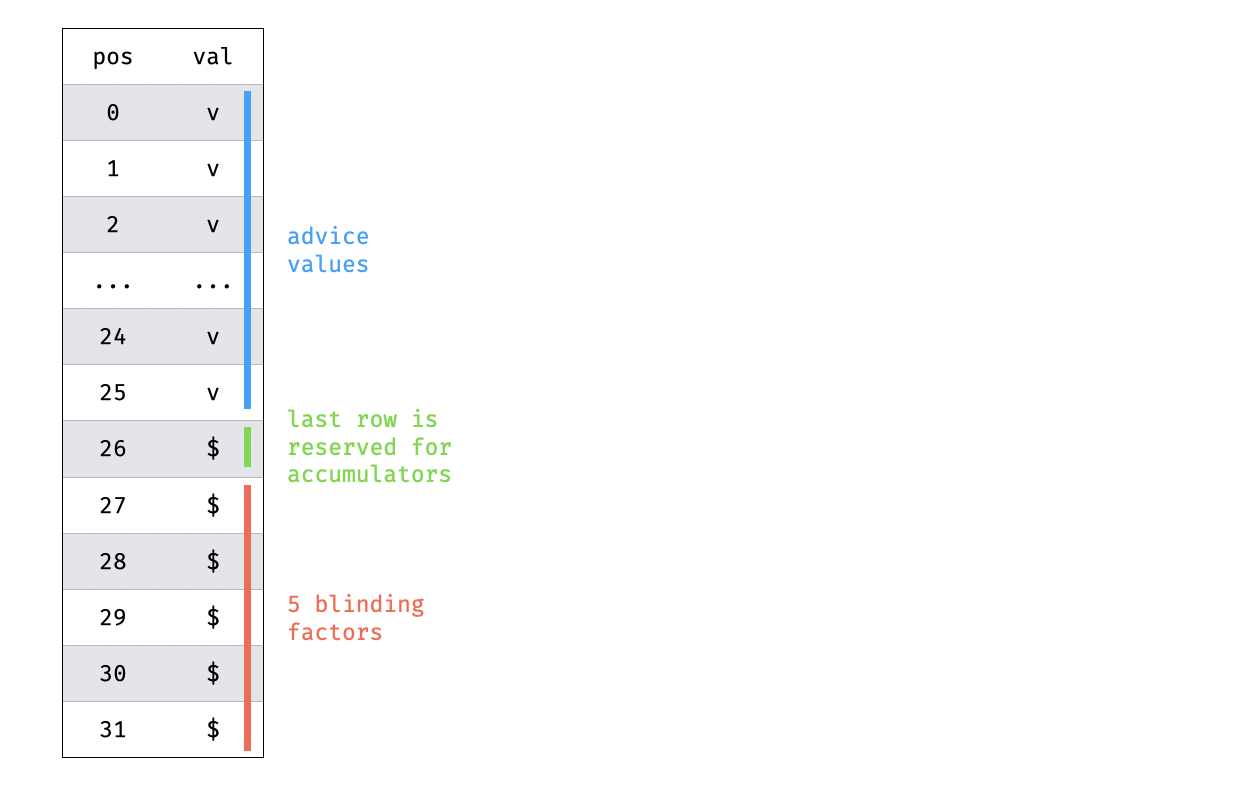
We have verified that this last row is correctly accounted in other parts of the protocol. This is important because no lookup or custom gate constraints can be applied there.

You can see the blinding of these $z$ polynomials implemented in src/plonk/permutation/prover.rs:

impl Argument {
    #[allow(clippy::too_many_arguments)]
    pub(in crate::plonk) fn commit<
        F: WithSmallOrderMulGroup<3>,
        CS: PolynomialCommitmentScheme<F>,
        R: RngCore,
        T: Transcript,
    >(
        &self,
        params: &CS::Parameters,
        pk: &plonk::ProvingKey<F, CS>,
        pkey: &ProvingKey<F>,
        advice: &[Polynomial<F, LagrangeCoeff>],
        fixed: &[Polynomial<F, LagrangeCoeff>],
        instance: &[Polynomial<F, LagrangeCoeff>],
        beta: F,
        gamma: F,
        mut rng: R,
        transcript: &mut T,
    ) -> Result<Committed<F>, Error>
    where
        CS::Commitment: Hashable<T::Hash>,
    {
        let domain = &pk.vk.domain;

        // How many columns can be included in a single permutation polynomial?
        // We need to multiply by z(X) and (1 - (l_last(X) + l_blind(X))). This
        // will never underflow because of the requirement of at least a degree
        // 3 circuit for the permutation argument.
        assert!(pk.vk.cs_degree >= 3);
        let chunk_len = pk.vk.cs_degree - 2;
        let blinding_factors = pk.vk.cs.blinding_factors();

        // TRUNCATED...

        for (columns, permutations) in self
            .columns
            .chunks(chunk_len)
            .zip(pkey.permutations.chunks(chunk_len))
        {

            // TRUNCATED...

            // Set blinding factors
            for z in &mut z[domain.n as usize - blinding_factors..] {
                *z = F::random(&mut rng);
            }
            // Set new last_z
            last_z = z[domain.n as usize - (blinding_factors + 1)];

Lookup Permutation Column

The lookup uses three new columns: a permutation column that reuses the same blinded layout as the above $z$ polynomials:

impl<F: WithSmallOrderMulGroup<3>> Permuted<F> {
    pub(in crate::plonk) fn commit_product<CS: PolynomialCommitmentScheme<F>, T: Transcript>(
        self,
        pk: &ProvingKey<F, CS>,
        params: &CS::Parameters,
        beta: F,
        gamma: F,
        mut rng: impl RngCore + CryptoRng,
        transcript: &mut T,
    ) -> Result<Committed<F>, Error>
    where
        F: WithSmallOrderMulGroup<3> + FromUniformBytes<64>,
        CS::Commitment: Hashable<T::Hash>,
    {
        let blinding_factors = pk.vk.cs.blinding_factors();

        // TRUNCATED...

        let z = iter::once(F::ONE)
            .chain(lookup_product)
            .scan(F::ONE, |state, cur| {
                *state *= &cur;
                Some(*state)
            })
            // Take all rows including the "last" row which should
            // be a boolean (and ideally 1, else soundness is broken)
            .take(pk.vk.n() as usize - blinding_factors)
            // Chain random blinding factors.
            .chain((0..blinding_factors).map(|_| F::random(&mut rng)))
            .collect::<Vec<_>>();
        assert_eq!(z.len(), pk.vk.n() as usize);

        // TRUNCATED...
    }
}

and two columns which are permutations of both the lookups and the lookup tables as you can see in the following diagram:

lookups

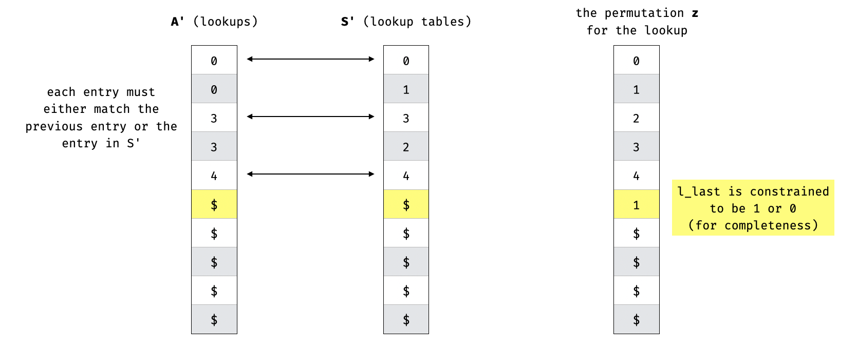
The blinding of these columns is implemented in src/plonk/lookup/prover.rs:

fn permute_expression_pair<F, CS: PolynomialCommitmentScheme<F>, R: RngCore>(
    pk: &ProvingKey<F, CS>,
    domain: &EvaluationDomain<F>,
    mut rng: R,
    input_expression: &Polynomial<F, LagrangeCoeff>,
    table_expression: &Polynomial<F, LagrangeCoeff>,
) -> Result<ExpressionPair<F>, Error>
where
    F: WithSmallOrderMulGroup<3> + Ord + FromUniformBytes<64>,
{
    let blinding_factors = pk.vk.cs.blinding_factors();
    let usable_rows = pk.vk.n() as usize - (blinding_factors + 1);

    // TRUNCATED...

    permuted_input_expression.extend((0..(blinding_factors + 1)).map(|_| F::random(&mut rng)));
    permuted_table_coeffs.extend((0..(blinding_factors + 1)).map(|_| F::random(&mut rng)));
    assert_eq!(permuted_input_expression.len(), pk.vk.n() as usize);
    assert_eq!(permuted_table_coeffs.len(), pk.vk.n() as usize);

    // TRUNCATED...
}

Blinding Factors For Quotient Polynomials

Quotient polynomials can be seen as separate columns in the protocol that are derived from the witness columns. For this reason, they must also be blinded in order to prevent information leakage.

As pointed out in Zero-Knowledge Is Not Fully Implemented this was not done properly.

Use of Coset for Polynomial Evaluation Overview

In Halo2, when evaluating polynomials over an extended domain to accommodate multiplication gates, the polynomial’s evaluations, initially defined over the original domain, are interpolated into coefficients and then re-evaluated over the extended domain. This would normally be done using a multiplicative subgroup of the extended domain. However, Halo2 instead uses a coset of the extended domain’s multiplicative subgroup to avoid division-by-zero errors.

Division-by-zero Errors

Halo2 performs operations on polynomials in evaluation form, and to compute the quotient polynomial $q (X)$ , it divides the constraint polynomial $h (X)$ by the vanishing polynomial $z (X)$ :

q (X) = \frac{h (X)}{z (X)}

By definition, the vanishing polynomial evaluates to zero over the original domain, and since the extended domain contains the original domain, this means that when computing the quotient polynomial, division by zero would occur. To prevent this issue, Halo2 uses a coset.

How a Coset Is Created

One way to create a coset of a multiplicative subgroup is to multiply each element in the subgroup by a scalar value that is not in the subgroup. If the scalar value is in the subgroup, the new set of values will be the same multiplicative subgroup.

Since Halo2 uses a subgroup of size $2^{k}$ (i.e., some power of 2) to efficiently perform FFT, one can simply find a subgroup of size $s$ that does not divide $2^{k}$ and use an element of that subgroup as the scalar value.

Specifically, Halo2 uses the generator $ζ$ of a multiplicative subgroup that has size $3$ and is composed of the following elements: ${ζ^{0}, ζ^{1}, ζ^{2}}$ .

Thus, given a multiplicative subgroup $G$ of size $2^{k}$ , we can create a coset $G^{'}$ by multiplying each element in $G$ by $ζ$ :

G^{'} = {ζ \cdot ω^{i} ∣ i \in [2^{k}]} .

Evaluating Polynomials Over a Coset

When evaluating the polynomials over the given coset, Halo2 uses a slight modification to apply the standard FFT algorithm, which expects to evaluate over a multiplicative subgroup, not a coset.

Specifically, instead of multiplying all the evaluation points by $ζ$ , Halo2 multiplies the coefficients of the polynomial by ${ζ^{0}, ζ^{1}, ζ^{2} \dots}$ and then performs FFT over the multiplicative subgroup.

For example, suppose we have a polynomial:

f (X) = a_{0} + a_{1} X + \dots + a_{n - 1} X^{n - 1},

and we want to evaluate it over the coset $G^{'}$ . We get:

f (ζ \cdot X) = a_{0} + a_{1} (ζ \cdot X) + (ζ \cdot X)^{2} + \dots + a_{n - 1} (ζ \cdot X)^{n - 1},

which simplifies to:

a_{0} + a_{1} (ζ \cdot X) + a_{2} (ζ^{2} \cdot X^{2}) + \dots + a_{n - 1} (ζ^{n - 1} \cdot X^{n - 1}) .

Since $ζ^{3} = 1$ and $ζ^{2} = ζ^{- 1}$ , we can substitute the powers of $ζ$ :

a_{0} + a_{1} (ζ \cdot X) + a_{2} (ζ^{- 1} \cdot X^{2}) + \dots + a_{n - 1} (ζ^{- 1} \cdot X^{n - 1}) .

assuming $n \mod 3 = 0$ .

We can also group the coefficients with the powers of $ζ$ so that we can express $f (X)$ as:

(ζ^{0} \cdot a_{0}) + (ζ^{1} \cdot a_{1}) X + (ζ^{- 1} \cdot a_{2}) X^{2} + \dots + (ζ^{- 1} \cdot a_{n - 1}) X^{n - 1},

which means we can multiply each coefficient by one of ${ζ^{0}, ζ^{1}, ζ^{- 1}}$ , then perform FFT over the multiplicative subgroup $G$ to obtain the same result as evaluating $f (X)$ over $G^{'}$ .

Findings

Below are listed the findings found during the engagement. High severity findings can be seen as so-called "priority 0" issues that need fixing (potentially urgently). Medium severity findings are most often serious findings that have less impact (or are harder to exploit) than high-severity findings. Low severity findings are most often exploitable in contrived scenarios, if at all, but still warrant reflection. Findings marked as informational are general comments that did not fit any of the other criteria.

High

#00 Zero-Knowledge Is Not Fully Implemented src/plonk #01 Duplicate KZG Queries Will Introduce Soundness and Completeness Issues src/poly/kzg/mod.rs

Medium

#02 Different Instances Can be Absorbed as Identical Transcripts src/plonk/verifier.rs #03 Missing Restriction on Rotation Value May Introduce Soundness Issues for Certain Circuits src/poly/mod.rs

Low

#04 Incorrect Calculation of the Cost Model dev/cost_model.rs #05 Inconsistent Behavior in Polynomial Multiplication src/poly/mod.rs #06 Proof Transcript Trailing Bytes Are Allowed src/plonk/verifier.rs #07 Fiat-Shamir Absorption of the Verifier Key is Fragile src/plonk

Informational

#08 Lagrange Interpolation Should Check for Duplicate Points src/utils/arithmetic.rs #09 Avoid Zero Representation for the Verifier Key src/plonk

High · #00

Zero-Knowledge Is Not Fully Implemented

src/plonk

Description. In order to provide zero-knowledge, the protocol has to blind committed polynomials that contain private data and that are evaluated as part of the protocol.

As each evaluation provides information about the underlying polynomial, the general rule is to add one degree of freedom to the polynomial for each evaluation.

Midnight’s Halo2 fork takes a departure from both the PSE fork and the zcash fork by providing evaluations for all committed polynomials, which allows the verifier to perform the plonk check in the clear.

That is, they perform the following check in the clear, given evaluations of these polynomials at a random challenge $x$ :

f (x) = Z_{H} (x) \cdot h (x)

where $f$ is the polynomial that aggregates all the constraints (custom gates, permutation, and lookup), $Z_{H}$ is the vanishing polynomial on the evaluation domain, and $h$ is the quotient polynomial.

While this approach makes sense, it also requires the prover to make sure that they correctly blind polynomials that were previously not being evaluated as part of the protocol.

This is the case for the quotient polynomial (called vanishing in the implementation) which is derived from other secret polynomials. This wouldn’t be a problem if the verifier would only get the evaluation of $h$ at the same challenge point $x$ because the verifier would not learn any new evaluation: they already can compute $h (x)$ themselves as $f (x) / Z_{H} (x)$ .

The problem is that, as with the vanilla plonk protocol, the implementation chunks $h$ into several polynomials, and then provides evaluations of these chunks. For example, we have the evaluations $h_{1} (x), h_{2} (x), h_{3} (x)$ , etc. such that $h (x) = h_{1} (x) + x^{n} \cdot h_{2} (x) + x^{2 n} \cdot h_{3} (x) + \dots$ .

This means that the attack on the zero-knowledge property of Plonk outlined in How (Not) to Simulate PLONK is feasible (in very contrived circuits).

Recommendation. We recommend fixing this by simply producing the expected evaluation $h (x) = f (x) / Z_{H} (x)$ and including it in the subsequent queries to verify via KZG evaluation proofs.

This would not only ensure that the chunks of $h$ are not evaluated, while ensuring that the later $h (x_{3})$ evaluation, provided as part of the multipoint opening protocol, remains zero-knowledge thanks to the random polynomial added in vanishing.

We talk about this in more detail in the Blinding Overview section.

Client Response. The issue was fixed in https://github.com/midnightntwrk/halo2/pull/3/commits/d4c4b9c4a526f84f2f55788a5cbea0da389cfe7f

High · #01

Duplicate KZG Queries Will Introduce Soundness and Completeness Issues

src/poly/kzg/mod.rs

Description. The KZG module supports verifying the openings of different polynomials/commitments and different points in one batch. However, it fails to handle duplicate queries (identical polynomials queried at the same point) and will introduce soundness and completeness issues.

In the code below, the construct_intermediate_sets function takes the sequence of all the queries and groups them by the query point. Due to an oversight, the function doesn’t consider the case that two queries may have the same polynomial and the same evaluation point. When that happens, the duplicate queries will be grouped together and the evaluation will be overwritten.

pub(super) type IntermediateSets<F, Q> = (
    Vec<CommitmentData<<Q as Query<F>>::Eval, <Q as Query<F>>::Commitment>>,
    Vec<Vec<F>>,
);

// Given a sequence of opening queries, group the query by points
pub fn construct_intermediate_sets<F: Field + Ord, I, Q: Query<F>>(
    queries: I,
) -> IntermediateSets<F, Q>
where
    I: IntoIterator<Item = Q> + Clone,
{
    // Construct sets of unique commitments and corresponding information about
    // their queries.
    let mut commitment_map: Vec<CommitmentData<Q::Eval, Q::Commitment>> = vec![];

    [...]

    // Initialise empty evals vec for each unique commitment
    for commitment_data in commitment_map.iter_mut() {
        let len = commitment_data.point_indices.len();
        commitment_data.evals = vec![Q::Eval::default(); len];
    }

    // For each query, update the evaluation in commitment_data
    for query in queries {
        [...]

        for commitment_data in commitment_map.iter_mut() {
            if query.get_commitment() == commitment_data.commitment {
                // Insert the evaluation using the ordering of the point_index_set
                // The issues here is that, when two queries have the same commitment and point, the evaluation will be overwritten
                commitment_data.evals[point_index_in_set] = query.get_eval();
            }
        }
    }

    [...]
}

The test below creates two queries that have the same polynomial and point but different evaluations. This is apparently a contradictory evaluation in the proof and should be rejected. However, after the processing, the two queries have the same evaluation. As a result, the contradictory evaluation is erased silently.

// add this test in src/poly/kzg/utils.rs
#[cfg(test)]
mod test {
    use crate::poly::query::Query;
    use ff::Field;
    use halo2curves::pasta::Fp;

    #[derive(Debug, Clone)]
    struct FakeQuery {
        point: Fp,
        commitment: Fp,
        eval: Fp,
    }

    impl FakeQuery {
        fn new(point: Fp, commitment: Fp, eval: Fp) -> Self {
            FakeQuery {
                point,
                commitment,
                eval
            }
        }
    }

    impl Query<Fp> for FakeQuery {
        type Commitment = Fp;
        type Eval = Fp;

        fn get_point(&self) -> Fp {
            self.point
        }

        fn get_commitment(&self) -> Fp {
            self.commitment
        }

        fn get_eval(&self) -> Fp {
            self.eval
        }
    }


    #[test]
    fn test_duplicate_query() {
        // q1 and q1 has the same commitment and point but different eval
        let q1 = FakeQuery::new(Fp::one(), Fp::one(), Fp::one() + Fp::one());
        let q2 = FakeQuery::new(Fp::one(), Fp::one(), Fp::ZERO);
        let (poly_map, point_sets) = super::construct_intermediate_sets(vec![q1, q2]);
        assert!(poly_map[0].evals[0] == poly_map[0].evals[1]); // the output has the same eval for the two queries
        println!("{:?}\n{:?}", poly_map, point_sets);
    }
}

The multi_prepare function calls the construct_intermediate_sets function and evaluates commitments that have identical query points in one group. If a commitment is queried at the same point x twice, it will be marked as having a single query point but two evaluations. For other commitments that are only queried once at x, they will have one evaluation. In the multi_prepare function they will be batched into one group (because they are only evaluated at x) but have different numbers of evaluations (because they are evaluated at x for different times).

fn multi_prepare<T: Transcript>(
    verifier_query: impl IntoIterator<Item = VerifierQuery<E::Fr, KZGCommitmentScheme<E>>> + Clone,
    transcript: &mut T,
) -> Result<DualMSM<E>, Error>
where
    E::Fr: Sampleable<T::Hash> + Ord + Hashable<T::Hash>,
    E::G1Affine: Hashable<T::Hash>,
{
    [...]
    let (commitment_map, point_sets) = construct_intermediate_sets(verifier_query);

    let mut q_coms: Vec<_> = vec![vec![]; point_sets.len()]; // commitment in q_coms[i][j] will be evaluated in point_sets[i] with q_eval_sets[i][j] as evaluations
    let mut q_eval_sets = vec![vec![]; point_sets.len()];

    for com_data in commitment_map.into_iter() {
        let mut msm = MSMKZG::new();
        msm.append_term(E::Fr::ONE, com_data.commitment.into());
        q_coms[com_data.set_index].push(msm);
        q_eval_sets[com_data.set_index].push(com_data.evals);
    }

    let q_coms = q_coms // compute q_coms = a_com + x1*b_com + x1^2*c_com + ...
        .iter()
        .map(|msms| {
            #[cfg(feature = "truncated-challenges")]
            let powers = truncated_powers(x1);

            #[cfg(not(feature = "truncated-challenges"))]
            let powers = powers(x1);

            msm_inner_product(msms, powers)
        })
        .collect::<Vec<_>>();

    let q_eval_sets = q_eval_sets // compute q_eval_sets = a_eval + x1*b_eval + x1^2*c_eval + ... (on the same eval point)
        .iter()
        .map(|evals| {
            #[cfg(feature = "truncated-challenges")]
            let powers = truncated_powers(x1);

            #[cfg(not(feature = "truncated-challenges"))]
            let powers = powers(x1);
            // Here, the crash occurs because the lengths of the evaluations are inconsistent.
            evals_inner_product(evals, powers)
        })
        .collect::<Vec<_>>();
    [...]
}


pub(crate) fn evals_inner_product<F: PrimeField + Clone>(
    evals_set: &[Vec<F>],
    scalars: impl Iterator<Item = F>,
) -> Vec<F> {
    // This assumes that all evaluations in evals_set have the same length.
    let mut res = vec![F::ZERO; evals_set[0].len()];
    for (poly_evals, s) in evals_set.iter().zip(scalars) {
        for i in 0..res.len() {
            res[i] += poly_evals[i] * s;
        }
    }
    res
}

In the evals_inner_product function above, it assumes each set in evals_set has the same length and then takes the length from the first set. As described above, this assumption doesn’t hold anymore when involved with duplicate KZG queries. If the length of the first set is larger than any of the others, then that will introduce out-of-bounds error and crash the verifier. This is a completeness issue and a DoS issue. On the other hand, if the length of the first set is shorter than the others, some evaluations will be ignored. This will introduce a soundness issue.

One might think that duplicate queries are unlikely to appear in a Halo2 proof. However, it turns out that it can happen in some cases:

Halo2 supports unblinded advice columns. If the witness has two unblinded advice columns with exactly the same values (either in one instance or across multiple instances), then the advice column polynomials/commitments will be the same. Then they will all be evaluated at the same point x.
If the circuit has two fixed columns with exactly the same values, then the column polynomials/commitments will be the same. Then the two polynomials will both be evaluated at the same point x. This should be less common in practice because duplicate fixed columns are useless.
A malicious prover can provide identical commitments for different polynomials, which will be evaluated at the same point x.

In the example below, we modify vector-ops-unblinded.rs to verify two identical proofs in one batch. As the advice column is unblinded, two identical instances will have the same column polynomial/commitment. This causes the verifier to crash due to the out-of-bounds array indexing error.

diff --git a/examples/vector-ops-unblinded.rs b/examples/vector-ops-unblinded.rs
index a7530ed2..4abbd222 100644
--- a/examples/vector-ops-unblinded.rs
+++ b/examples/vector-ops-unblinded.rs
@@ -356,7 +356,7 @@ impl<F: Field> NumericInstructions<F> for AddChip<F> {
     }
 }

-#[derive(Default)]
+#[derive(Default, Clone)]
 struct MulCircuit<F: Field> {
     a: Vec<Value<F>>,
     b: Vec<Value<F>>,
@@ -409,7 +409,7 @@ impl<F: Field> Circuit<F> for MulCircuit<F> {
 }
 // ANCHOR_END: circuit

-#[derive(Default)]
+#[derive(Default, Clone)]
 struct AddCircuit<F: Field> {
     a: Vec<Value<F>>,
     b: Vec<Value<F>>,
@@ -464,7 +464,7 @@ impl<F: Field> Circuit<F> for AddCircuit<F> {

 fn test_prover<E: Engine + MultiMillerLoop>(
     k: u32,
-    circuit: impl Circuit<E::Fr>,
+    circuit: impl Circuit<E::Fr> + Clone,
     expected: bool,
     instances: Vec<E::Fr>,
 ) -> Vec<u8>
@@ -487,8 +487,8 @@ where
         create_proof::<E::Fr, KZGCommitmentScheme<E>, _, _>(
             &params,
             &pk,
-            &[circuit],
-            &[&[&instances]],
+            &[circuit.clone(), circuit.clone()],
+            &[&[&instances], &[&instances]],
             OsRng,
             &mut transcript,
         )
@@ -500,7 +500,7 @@ where
     let accepted = {
         let mut transcript = CircuitTranscript::<State>::init_from_bytes(&proof[..]);

-        prepare::<E::Fr, KZGCommitmentScheme<E>, _>(pk.get_vk(), &[&[&instances]], &mut transcript)
+        prepare::<E::Fr, KZGCommitmentScheme<E>, _>(pk.get_vk(), &[&[&instances], &[&instances]], &mut transcript)
             .unwrap()
             .verify(&params.verifier_params())
     };

For the soundness issue, the prover can commit the random polynomial in Vanishing Argument to be equal to the second advice column polynomial. We assume that the column polynomial will only be evaluated one point x. Then, the two polynomials will be treated as the same polynomial and will be evaluated at the same x with two evaluations. The evals_inner_product function won’t crash because the polynomial (with duplicate query) is the second element and the first element only has only evaluation. Instead, the second evaluation will be ignored in the KZG check. That means the prover can set the second evaluation as an arbitrary value (without being caught by the KZG check) to satisfy the vanishing evaluation check. This introduces the soundness issue.

Impact. This is a soundness, completeness and DoS issue. A malicious prover can create bad proof with duplicate KZG queries to bypass the verifier check. The verifier may not able be to verify legal proofs that have identical commitments. A malicious prover can create a bad proof with duplicate queries to crash the verifier.

Recommendation. We noticed that the zcash-halo2 and pse-halo2 compare polynomial commitment by reference. In this way, two independent polynomials will always be treated as different items and won’t have duplicate queries, although they may have the same commitment value. It’s recommended to use a similar way to compare polynomial commitment by reference instead of by values.

Client Response. The issue was fixed in https://github.com/midnightntwrk/halo2/pull/3/commits/319af9befa3ce7ff79b759b7b54031b7f8a70ba1.

Medium · #02

Different Instances Can be Absorbed as Identical Transcripts

src/plonk/verifier.rs

Description. The Halo2 verifier supports batch verifying multiple instances (of the same circuit) in the prepare. The input instances is a 3-d array that can contain multiple circuit instances, each can have multiple instance columns and each column can have multiple values. The function absorbs all the instance values one-by-one without considering the array length and there is no restriction on the length of each column. This will lead to different instances being absorbed as identical transcripts and cause transcript collision.

pub fn prepare<F, CS: PolynomialCommitmentScheme<F>, T: Transcript>(
    vk: &VerifyingKey<F, CS>,
    instances: &[&[&[F]]],
    transcript: &mut T,
) -> Result<CS::VerificationGuard, Error>
where
    F: WithSmallOrderMulGroup<3>
        + Hashable<T::Hash>
        + Sampleable<T::Hash>
        + FromUniformBytes<64>
        + Ord,
    CS::Commitment: Hashable<T::Hash>,
{
    // Check that instances matches the expected number of instance columns
    for instances in instances.iter() {
        if instances.len() != vk.cs.num_instance_columns {
            return Err(Error::InvalidInstances);
        }
    }

    let num_proofs = instances.len();

    // Hash verification key into transcript
    vk.hash_into(transcript)?;

    for instance in instances.iter() {
        for instance in instance.iter() {
            for value in instance.iter() {
                transcript.common(value)?;
            }
        }
    }
    [...]
}

Consider these two different instances: A: [[[1, 2], [3]]], B: [[[1], [2, 3]]]. They will both be absorbed as the same sequence 1, 2, 3 and then generate the same transcript. This means that a prover can fix the transcript (along with all the challenges) and rearrange the input instances. A malicious prover can utilize this to fix the challenge and try different arrangements to see if they passes the later evaluation check.

In some cases, this might work. For example, suppose the canonical instances is [[[1, 2, 0], [0]]. The prover can rearrange that to be [[[1, 2], [0, 0]] and still pass the verification. This is because the new instances generates the same transcript and has the same evaluations with the canonical one. In this case, the underlying instance polynomials are still unchanged so this is not considered to be a soundness issue. Currently, it is unclear whether a prover can find (meaningful) distinct instance columns that both pass verification.

Impact. The length of each instance column is checked in a higher level api so this does not introduce vulnerabilities for midnight-circuit users. However this behavior is implicit and might cause issues for Midnight Halo2 users.

Recommendation. To prevent transcript collisions, it is recommended to include the length of each instance column in the transcript absorption process. Additionally, it’s recommended to add documentation in the prepare function and clarify that it’s the caller’s responsibility to check the length of the instance column.

Client Response. The issue was fixed in https://github.com/midnightntwrk/halo2/pull/3.

Medium · #03

Missing Restriction on Rotation Value May Introduce Soundness Issues for Certain Circuits

src/poly/mod.rs

Description. In Halo2, the Rotation represents the relative offset of the query. Currently, there is no restriction on the rotation value. This may introduce soundness issues or crash the verifier for some circuits.

The soundness issue arises from duplicate KZG queries. Suppose the k of the circuit is 4. The query of a column at Rotation::cur() and at Rotation(16) result in the same position because the latter warps. If a circuit has a gate that queries these two positions at the same column and finally they become identical query points of the same column (commitment). Below is an example of such a query:

// This gate will always be satisfied.
cs.create_gate("hack", |meta| {
    let cur = meta.query_advice(advice1, Rotation::cur());
    let cur_warpped = meta.query_advice(advice1, Rotation(16)); // This is the warped current row
    vec![cur - cur_warpped]
});

A circuit with the above gate will introduce duplicate queries of the same commitment. As described in Duplicated Query Finding, duplicate queries in KZG may introduce soundness and completeness issues in Halo2. This means that any circuit with the above query pattern is not sound. Moreover, a secure circuit can become insecure by simply adding a dummy query like this. Note that this issue also applies to the zcash-halo2 and pse-halo2 because it involves duplicate query point on the same column polynomial.

Besides, during verification, a vector l_i_s is computed as the evaluations of Lagrange basis polynomials over a range of rotations from -max_rotation up to (max_instance_len + |min_rotation|). A large or extreme rotation can inflate the size of l_i_s with redundant evaluations.

In an extreme edge case, something like Rotation(-i32::MAX) can trigger a negative overflow in release mode, yielding a zero-length l_i_s. The code then tries to slice l_i_s[offset..offset+instances.len()], causing a panic “index out of range.”. While this scenario is unlikely (as the proof generation in this extreme scenario would typically fail), it reveals a missing check that allows malicious or extremely large rotations to slip through.

Impact. The unrestricted rotation value may introduce a soundness issue or crash the verifier for some circuits.

Recommendation. It’s recommended to restrict the rotation value (e.g., within (-n/2, n/2)) during synthesizing to avoid potential issues.

Client Response. The issue was fixed in https://github.com/midnightntwrk/halo2/pull/3/commits/319af9befa3ce7ff79b759b7b54031b7f8a70ba1

Low · #04

Incorrect Calculation of the Cost Model

dev/cost_model.rs

Description. The cost model in dev/cost_model.rs calculates the cost of (e.g., proof size) a given circuit. Due to an oversight, some parts of the cost calculation are incorrect and deviate from the actual cost.

Here, only one commitment is added for the permutation argument. However, in the proof, the permutation product commitment is split into chunks based on the max degree and the number of permutation columns. As a result, there may be multiple product commitments.

Additionally, the permutation query point here is incorrect. Due to the presence of blinding rows, the last queried row of the product commitment is u instead of -1. Therefore, the actual query point should be “0, 1, u”.

Impact. This discrepancy causes the estimated cost to deviate from the actual cost.

Recommendation. It is recommended to correct the cost calculation according to the protocol to ensure accuracy.

Client Response. This was fixed in https://github.com/midnightntwrk/halo2/pull/2.

Low · #05

Inconsistent Behavior in Polynomial Multiplication

src/poly/mod.rs

Description. The Mul function multiplies a polynomial with a scalar. The expected behavior is to modify the polynomial and return self. However, when the scalar is F::ZERO, it will just create a zero polynomial and return it, without modifying the polynomial itself. The behavior is inconsistent across different cases.

impl<F: Field, B: Basis> Mul<F> for Polynomial<F, B> {
    type Output = Polynomial<F, B>;

    fn mul(mut self, rhs: F) -> Polynomial<F, B> {
        if rhs == F::ZERO {
            return Polynomial {
                values: vec![F::ZERO; self.len()],
                _marker: PhantomData,
            };
        }
        if rhs == F::ONE {
            return self;
        }

        parallelize(&mut self.values, |lhs, _| {
            for lhs in lhs.iter_mut() {
                *lhs *= rhs;
            }
        });

        self
    }
}

Impact. We didn’t find a direct security issue related to this but it may introduce subtle bugs in future development.

Recommendation. It’s recommended to remove the rhs == F::ZERO case.

Client Response. The issue was fixed in https://github.com/midnightntwrk/halo2/pull/3/commits/942ccba2677ed024c4791c7117476ce4c3cb60de

Low · #06

Proof Transcript Trailing Bytes Are Allowed

src/plonk/verifier.rs

Description. The prepare function of src/plonk/verifier.rs does not check if a transcript initialized with proof bytes contains extra bytes after all necessary reads from the transcript have been made. This allows a malicious prover to supply a proof with extra trailing bytes. Consider the following test case (built after defining an example circuit which we omit for brevity):

    ...
   let proof = prover_transcript.finalize();
    println!("Proof length: {}", proof.len());


    // Append some arbitrary bytes.
    let mut tampered_proof = proof.clone();
    tampered_proof.extend_from_slice(&[0u8; 10]);

    println!("Tampered proof length: {}", tampered_proof.len());
    let mut verifier_transcript = CircuitTranscript::<_>::init_from_bytes(&tampered_proof);

    let guard = prepare::<Fr, KZGCommitmentScheme<Bn256>, _>(
        &vk,
        &[&[&public_instances[0]]],
        &mut verifier_transcript,
    )
    .expect("proof preparation should succeed");

    assert!(guard.verify(&params.verifier_params()).is_ok());
    println!("Proof verified successfully.");

This outputs:

Proof length: 1184
Tampered proof length: 1194
Proof verified successfully.

Although this manipulation of the proof is not immediately a soundness concern and there is currently no obvious exploit, in cryptographic protocols it is considered a best practice to strictly enforce the expected transcript format, and in particular, check for extra trailing bytes. For instance the Ethereum specification recommends to check for trailing bytes in transactions after decoding. CVE-2018-16150 arises due to permissiveness on the trailing bytes. Strict format checks have been advocated for Fiat-Shamir transcripts due to several recent bugs found in implementations.

Recommendation. It is recommended that the verifier checks if all bytes of a proof transcript have been read, and potentially triggers and error and rejects a proof if there are extra bytes remaining. If it is intended to have extra bytes in the proof to include meta-data or other information, this should be documented in the code.

Client response. The issue was fixed in https://github.com/midnightntwrk/halo2/pull/3.

Low · #07

Fiat-Shamir Absorption of the Verifier Key is Fragile

src/plonk

Description. The first step in the Fiat-Shamirization of the Halo2 Plonk implementation is to absorb the verifier key. This step is done by both the prover and the verifier. For example, in src/plonk/verifier.rs:

/// Prepares a plonk proof into a PCS instance that can be finalized or batched.
pub fn prepare<F, CS: PolynomialCommitmentScheme<F>, T: Transcript>(
    vk: &VerifyingKey<F, CS>,
    instances: &[&[&[F]]],
    transcript: &mut T,
) -> Result<CS::VerificationGuard, Error>
where
    F: WithSmallOrderMulGroup<3>
        + Hashable<T::Hash>
        + Sampleable<T::Hash>
        + FromUniformBytes<64>
        + Ord,
    CS::Commitment: Hashable<T::Hash>,
{
    // TRUNCATED...

    // Hash verification key into transcript
    vk.hash_into(transcript)?;

This field is set in the from_parts() function that is always called:

impl<F: WithSmallOrderMulGroup<3>, CS: PolynomialCommitmentScheme<F>> VerifyingKey<F, CS> {
    fn from_parts(
        domain: EvaluationDomain<F>,
        fixed_commitments: Vec<CS::Commitment>,
        permutation: permutation::VerifyingKey<F, CS>,
        cs: ConstraintSystem<F>,
    ) -> Self
    where
        F: FromUniformBytes<64>,
    {
        // TRUNCATED...
        let mut vk = Self {
            // TRUNCATED...
            transcript_repr: F::ZERO,
        };

        let mut hasher = Blake2bParams::new()
            .hash_length(64)
            .personal(b"Halo2-Verify-Key")
            .to_state();

        let s = format!("{:?}", vk.pinned());

        hasher.update(&(s.len() as u64).to_le_bytes());
        hasher.update(s.as_bytes());

        // Hash in final Blake2bState
        vk.transcript_repr = F::from_uniform_bytes(hasher.finalize().as_array());

        vk
    }

One potential issue is in the following line:

let s = format!("{:?}", vk.pinned());

which produces the string to be hashed via the Debug implementation of a structure. In practice, it ends up relying on Debug implementations all the way down, down to how specific types implement their Debug trait in crates like pairing and bn256. For example:

vk-pinned

The issue is that it is a fragile way to hash the verifier key, as it relies on the correctness of the Debug implementations of all the types involved.

Not only is it common to see code changes that override the default Debug implementation in order to truncate or shorten what is output in order to facilitate debugging, it also makes the introduction of new polynomial commitment schemes or new crates in this path a potential venue for new bugs or even a new attack vector for a supply chain attack.

Furthermore, some of the Debug implementations are custom, and it’s not always immediately clear that they are including all of the important fields (as opposed to a default Debug implementation). For example:

impl<'a, F: Field> std::fmt::Debug for PinnedConstraintSystem<'a, F> {
    fn fmt(&self, f: &mut std::fmt::Formatter<'_>) -> std::fmt::Result {
        let mut debug_struct = f.debug_struct("PinnedConstraintSystem");
        debug_struct
            .field("num_fixed_columns", self.num_fixed_columns)
            .field("num_advice_columns", self.num_advice_columns)
            .field("num_instance_columns", self.num_instance_columns)
            .field("num_selectors", self.num_selectors);
        // Only show multi-phase related fields if it's used.
        if *self.num_challenges > 0 {
            debug_struct
                .field("num_challenges", self.num_challenges)
                .field("advice_column_phase", self.advice_column_phase)
                .field("challenge_phase", self.challenge_phase);
        }
        debug_struct
            .field("gates", &self.gates)
            .field("advice_queries", self.advice_queries)
            .field("instance_queries", self.instance_queries)
            .field("fixed_queries", self.fixed_queries)
            .field("permutation", self.permutation)
            .field("lookups", self.lookups);
        debug_struct
            .field("constants", self.constants)
            .field("minimum_degree", self.minimum_degree);
        debug_struct.finish()
    }
}

Recommendation. A better way of writing the above snippet in order to leverage compiler warnings would be to deconstruct the value before using its fields:

impl<'a, F: Field> std::fmt::Debug for PinnedConstraintSystem<'a, F> {
    fn fmt(&self, f: &mut std::fmt::Formatter<'_>) -> std::fmt::Result {
        let &Self {
            num_fixed_columns,
            num_advice_columns,
            num_instance_columns,
            num_selectors,
            num_challenges,
            advice_column_phase,
            challenge_phase,
            gates,
            advice_queries,
            instance_queries,
            fixed_queries,
            permutation,
            lookups,
            constants,
            minimum_degree,
        } = &self;
        let mut debug_struct = f.debug_struct("PinnedConstraintSystem");
        debug_struct
            .field("num_fixed_columns", num_fixed_columns)
            .field("num_advice_columns", num_advice_columns)
            .field("num_instance_columns", num_instance_columns)
            .field("num_selectors", num_selectors);
        // Only show multi-phase related fields if it's used.
        if *num_challenges > &0 {
            debug_struct
                .field("num_challenges", num_challenges)
                .field("advice_column_phase", advice_column_phase)
                .field("challenge_phase", challenge_phase);
        }
        debug_struct
            .field("gates", &gates)
            .field("advice_queries", advice_queries)
            .field("instance_queries", instance_queries)
            .field("fixed_queries", fixed_queries)
            .field("permutation", permutation)
            .field("lookups", lookups);
        debug_struct
            .field("constants", constants)
            .field("minimum_degree", minimum_degree);
        debug_struct.finish()
    }
}

Furthermore, we recommend not relying on the output of the Debug implementations to encode the verifier key as it is generally intended for debugging purposes.

Client Response. The client acknowledged this issue.

Informational · #08

Lagrange Interpolation Should Check for Duplicate Points

src/utils/arithmetic.rs

Description. The function lagrange_interpolate in src/utils/arithmetic.rs is expected to panic when two points are repeated on the input points, according to the description of the function:

/// Returns coefficients of an n - 1 degree polynomial given a set of n points
/// and their evaluations. This function will panic if two values in `points`
/// are the same.
pub fn lagrange_interpolate<F: Field>(points: &[F], evals: &[F]) -> Vec<F> {

However this check is not implemented and when tested with 2 such repeated points the function outputs an empty polynomial and no errors. This is not currently exploitable because this function is called only in src/poly/kzg/mod.rs after getting the points from construct_intermediate_sets which by construction uses BTreeSet, ruling out duplicates. However it could be come an issue in a refactor if the function is called elsewhere and no checks are performed on the input points.

Recommendation. It is recommended that either checks are implemented for duplicates in the points input, or the documentation is changed to specify that this must be checked before calling the function.

Client response. The issue was fixed in https://github.com/midnightntwrk/halo2/pull/3.

Informational · #0a

Avoid Zero Representation for the Verifier Key

src/plonk

Description. As part of verifying a proof, a single field element (called transcript_repr) is created from the verifier key and absorbed in the transcript. You can see this in src/plonk/mod.rs:

pub struct VerifyingKey<F: PrimeField, CS: PolynomialCommitmentScheme<F>> {
    // TRUNCATED...
    transcript_repr: F,
}

impl<F: WithSmallOrderMulGroup<3>, CS: PolynomialCommitmentScheme<F>> VerifyingKey<F, CS> {
    pub fn hash_into<T: Transcript>(&self, transcript: &mut T) -> io::Result<()>
    where
        F: Hashable<T::Hash>,
    {
        transcript.common(&self.transcript_repr)?;

        Ok(())
    }

This single field element is initialized to zero, then later it is set to a BLAKE2b hash of the verifier key by calling VerifyingKey::from_parts(). We discuss this in more detail in Fiat-Shamir Absorption of the Verifier Key is Fragile.

It is important that the verifier key can never be initialized in a way that the transcript_repr field is never updated and remains zero (i.e. from_parts() is not called). If this happens, the verifier key will be absorbed as zero in the transcript, which can lead to a Fiat-Shamir bug.

While we could not find a way to construct such an invalid verifying key, it would be safer to make the code resistant to refactorings or API changes that could introduce a Fiat-Shamir bug.

Recommendation. We recommend using a memoization technique to force the value of the transcript_repr field to be computed (only once) when being read. This can be done with the OnceCell type, for example.

← Back to Index