Audit of Midnight Foreign Field, ECC & Hashing Circuits

Introduction

On November 18th, 2024, zkSecurity was commissioned to perform a security audit of IOG’s circuits for the Midnight network at commit dec9e46; this code originally resided in an internal repository and was archived in the new repository prior to publication for transparency and future reference.

For the two weeks, four consultants reviewed the Midnight circuits written in Halo2 in search of bugs. Further, starting on January 6th, 2025, two consultants focused on the SHA256 implementation for one additional week to cover the full scope. A number of observations and findings have been reported to the IOG team. The findings are detailed in the latter section of this report.

The Midnight circuits were found to be of high quality, accompanied by thorough documentation and tests.

Note that security audits are a valuable tool for identifying and mitigating security risks, but they are not a guarantee of perfect security. Security is a continuous process, and organizations should always be working to improve their security posture.

Scope

The scope of the audit was divided into distinct parts:

• Non-Native Arithmetic / Foreign Field Arithmetic Circuits (src/field).
• Other Circuit Gadgets, including:
  • Two SHA-256 circuits targeting different circuit sizes, using different lookup table sizes (src/sha256).
  • Poseidon Circuit (src/poseidon).
  • Elliptic Curve Arithmetic, covering both native (supporting an inner Edwards curve) and foreign/non-native implementations, as well as the hash-to-curve circuit (src/ecc).
  • Merkle Tree Circuit (src/map), including a membership verifier (examples/membership.rs).
  • A gadget for emulating arithmetic over large unsigned integers (src/biguint).

Additionally, we reviewed the API provided by the Midnight library (src/compact_std_lib.rs and src/instructions).

Background on Midnight Circuits

This section provides an overview of the Midnight library and circuits.

Overview of the Midnight Library

Midnight Circuits is a library designed for implementing circuits with Halo2. It is built on the PSE v0.4.0 release of the Halo2 fork. Midnight Circuits provides a variety of gadgets to build upon, including:

• Native and non-native field operations.
• Native and non-native elliptic-curve operations.
• Arithmetic over large unsigned integers.
• Native hash-to-curve operations.
• SHA256 and Poseidon hashing operations.
• Membership operations based on a Merkle tree implementation.

All of these functionalities are exposed as gadgets in src/compact_std_lib.rs, with their APIs defined in the traits located in src/instructions.

Using Midnight Circuits is straightforward, and numerous examples can be found in the examples/ directory. However, users should take care to properly constrain the value cells passed to Midnight Circuits (e.g., via std_lib.assign_many) and ensure that values computed by Midnight Circuits and exposed as public inputs are correctly constrained (e.g., using std_lib.constrain_as_public_input).

Range Checks

Range checks enforce that a field element $x\in {𝔽}_p$ belongs to a set of values $\{0,1,2,\dots ,B\}\subseteq {𝔽}_p$, i.e. it is “small”. For instance, in the foreign field emulation code, range checks ensure that the limbs of a field element are in the range $[0,B)$ and that integer relations being checked do not overflow the modulus of the field. Let us describe how range checks are implemented in the Midnight circuits.

Pow2RangeChip

The Pow2RangeChip chip handles range checking cells in small power-of-two ranges. The ranges must be small (e.g. 8-bits) since the range check uses a lookup table: a table contains all values from the range and a range check simply verifies that the value appears in the table. To support multiple ranges (all powers of two smaller than some max_bit_len), a “table” is created for each. To avoid allocating many columns, all tables are packed into a single larger table with rows separated by a “tag”, resulting in:

In other words, checking that $(b,\mathsf{a}\mathsf{s}\mathsf{s}\mathsf{i}\mathsf{g}\mathsf{n}\mathsf{e}\mathsf{d}\mathsf{\_}\mathsf{l}\mathsf{i}\mathsf{m}\mathsf{b})\in T$ implies $\mathsf{a}\mathsf{s}\mathsf{s}\mathsf{i}\mathsf{g}\mathsf{n}\mathsf{e}\mathsf{d}\mathsf{\_}\mathsf{l}\mathsf{i}\mathsf{m}\mathsf{b}\in \{0,1,\dots ,2^b-1\}\subseteq {𝔽}_p$.

The actual lookup constraint enforces a “vectorized” version of this lookup, checking that a vector of values $(b,{\mathsf{a}\mathsf{s}\mathsf{s}\mathsf{i}\mathsf{g}\mathsf{n}\mathsf{e}\mathsf{d}\mathsf{\_}\mathsf{l}\mathsf{i}\mathsf{m}\mathsf{b}}_1,{\mathsf{a}\mathsf{s}\mathsf{s}\mathsf{i}\mathsf{g}\mathsf{n}\mathsf{e}\mathsf{d}\mathsf{\_}\mathsf{l}\mathsf{i}\mathsf{m}\mathsf{b}}_2,{\mathsf{a}\mathsf{s}\mathsf{s}\mathsf{i}\mathsf{g}\mathsf{n}\mathsf{e}\mathsf{d}\mathsf{\_}\mathsf{l}\mathsf{i}\mathsf{m}\mathsf{b}}_3,{\mathsf{a}\mathsf{s}\mathsf{s}\mathsf{i}\mathsf{g}\mathsf{n}\mathsf{e}\mathsf{d}\mathsf{\_}\mathsf{l}\mathsf{i}\mathsf{m}\mathsf{b}}_4)$ satisfies:

Note that the same range is enforced on all the values. This is implemented by the “pow2range column check”:

for val_col in val_cols {
    meta.lookup("pow2range column check", |meta| {
        let sel = meta.query_selector(q_pow2range);
        let tag = meta.query_fixed(tag_col, Rotation::cur());
        let val = meta.query_advice(val_col, Rotation::cur());
        vec![(tag, t_tag), (sel * val, t_val)]
    });
}

The lookup is “disabled” (made trivial) when tag = q_pow2range = 0, causing a lookup of the dummy all-zeroes vector in the first table row. Note that the sub-table separators must be unique within the tag column if this lookup column is shared with another chip. In the code, the column is used exclusively by the Pow2RangeChip.

P2RDecompositionChip

The P2RDecompositionChip uses the Pow2RangeChip to combine multiple smaller range checks using linear combinations (see the native chip section) for checking larger ranges. This is implemented by “superimposing” the Pow2RangeChip on top of the NativeChip— enabling both gates at the same offset.

By configuring the NativeChip to compute a linear combination of the limbs with coefficients $1,B,B^2,B^3$ and enabling the Pow2RangeChip at the same offset with a tag for range $[0,B)$, we can verify that the linear combination is in range $[0,B^4)$:

Smaller Range: For smaller ranges (with fewer than 4 limbs), we simply set the coefficients of unused limbs to zero in the linear combination. For example, for a range $[0,B)$ with 3 limbs the linear combination is: $\mathsf{a}\mathsf{s}\mathsf{s}\mathsf{i}\mathsf{g}\mathsf{n}\mathsf{e}\mathsf{d}\mathsf{\_}\mathsf{r}\mathsf{e}\mathsf{s}\mathsf{u}\mathsf{l}\mathsf{t}={\mathsf{a}\mathsf{s}\mathsf{s}\mathsf{i}\mathsf{g}\mathsf{n}\mathsf{e}\mathsf{d}\mathsf{\_}\mathsf{l}\mathsf{i}\mathsf{m}\mathsf{b}\mathsf{s}}_0+B·{\mathsf{a}\mathsf{s}\mathsf{s}\mathsf{i}\mathsf{g}\mathsf{n}\mathsf{e}\mathsf{d}\mathsf{\_}\mathsf{l}\mathsf{i}\mathsf{m}\mathsf{b}\mathsf{s}}_1+B^2·{\mathsf{a}\mathsf{s}\mathsf{s}\mathsf{i}\mathsf{g}\mathsf{n}\mathsf{e}\mathsf{d}\mathsf{\_}\mathsf{l}\mathsf{i}\mathsf{m}\mathsf{b}\mathsf{s}}_2$.

This technique works for proving ranges $[0,B^k)$ where $k\le 4$. For larger ranges, or ranges with a bit-size not divisible by $b$ where $B=2^b$, we extend the technique to split the range check across multiple rows with different bounds $B$. This works well since the native gate supports carrying between rows, allowing longer linear combinations across multiple rows without copy constraints. The implementation is:

// assign terms for linear combination
let native_chip = self.native_chip();
let (assigned_limbs, assigned_result) = native_chip.assign_linear_combination_aux(
    &mut region,
    terms.as_slice(),
    F::ZERO,
    &x,
    NB_POW2RANGE_COLS,
    &mut offset,
)?;
offset += 1;

// enable the appropriate copy constraints in the rows where we assigned the
// linear combination terms
let pow2range_chip = self.pow2range_chip();

// get the lookup selector and tag columns
let range_selector_column = pow2range_chip.config().q_pow2range;
let range_tag_column = pow2range_chip.config().tag_col;

// we reverse since we do the rangechecks from higher end to start
for (i, tag) in tags.into_iter().rev().enumerate() {
    let current_row = offset - (i + 1);
    range_selector_column.enable(&mut region, current_row)?;
    region.assign_fixed(
        || "assign decomposition tag",
        range_tag_column,
        current_row,
        || Value::known(F::from(tag as u64)),
    )?;
}

The final task is computing the optimal number of rows needed to enforce the range. This is done using a dynamic programming algorithm that calculates the optimal decomposition for increasingly larger ranges, beginning with ranges enforceable in a single row.

Native Field

Native Chip

The native chip implements common arithmetic operations over the native field. This is accomplished using one custom gate which checks the following relation

q_arith * (
    (sum_i coeff[i] * values[i])
    + q_next * value[0].next +
    + mul_ab * value[0] * value[1] +
    + mul_cd * value[2] * value[3] +
    + constant
) = 0

where values are stored in advice columns, and all the other terms are stored in fixed columns, and values[0].next is the value in the values[0] column at the next row. The length of the values and coeffs array is a constant, and it is set to 5 in the current implementation.

pub const NB_ARITH_COLS: usize = 5;

By customizing the fixed terms, this gate is specialized to implement a lot of common arithmetic operations over the native field, which are used extensively throughout the library.

A lot of those operations eventually call into the custom() function, which implements a general application of the gate. It assigns all the fixed values over some input region and enables the q_arith selector to enforce the constraint in the current region at the given offset.

Most of the operations are quite straight forward, but it is worth mentioning how the circuit can assert the result of a linear combination. This is accomplished by the function linear_combination(), which calls into theassign_linear_combination_aux() function. Given some coefficients, values, a constant and a result it asserts that:

Since the length of the linear combination is arbitrary, this is accomplished using the custom gate over multiple rows, each row checking one part of the linear combination. We decompose the sum into two parts, first computing the first $K$ terms, and then checking the rest:

Notice that checking the remaining linear combination is a smaller instance of the original problem. We enforce the constraints over the rows recursively as follows, using the linear combination part of the custom gate and taking $K$ to be the number of columns in the gate minus one.

-res[0] + res[1] + c[0]*a[0] + c[1]*a[1] + ... + c[K-1]*a[K-1] = 0
-res[1] + res[2] + c[K]*a[K] + c[K+1]*a[K+1] + ... + c[2*K-1]*a[2*K-1] = 0
...
-res[L] + c[L*K]*a[L*K] + c[L*K+1]*a[L*K+1] [+ ...] = 0

At some point the number of remaining terms to check fit in one row, and we can check the relation directly with one application of the custom gate. The current result is stored in the first value column, and the result in the next row is retrieved by setting q_next to one. The constant is only added into the relation on the top-level call, all other recursive calls have the constant term set to zero.

NativeGadget

The NativeGadget is a gadget that combines a CoreDecomposition and a NativeArith chips to provide common functionalities, like range checks, comparisons and decomposition of field elements. As before, most functions are straight-forward, but it is worth mentioning how the assert_lower_than_fixed() function works. This asserts that some assigned native is lower than a given constant bound. The core decomposition chip provides a assert_less_than_pow2() function, which range checks some value in the range $[0,2^t)$ for some $t$. Checking that a number belongs to some arbitrary range $[0,b)$ where $b\in [2^k,2^{k+1})$ is equivalent to check that

The prover witnesses the bit $b$, that indicates which relation they want to prove. Then they prove a valid range check with the corresponding power of two.

Two other functions worth mentioning are lower_than() and lower_than_fixed(), which return true if the given bounded element is strictly less than another field element. We know that a bounded element (at the type-system level) has some bound $2^{\mathsf{b}\mathsf{o}\mathsf{u}\mathsf{n}\mathsf{d}}$, so if $y\ge 2^{\mathsf{b}\mathsf{o}\mathsf{u}\mathsf{n}\mathsf{d}}$ then the function returns true. ($x<2^{\mathsf{b}\mathsf{o}\mathsf{u}\mathsf{n}\mathsf{d}}\le y$). Otherwise, we know that $y<2^{\mathsf{b}\mathsf{o}\mathsf{u}\mathsf{n}\mathsf{d}}$. - If $x<y$ then $y-x>0$, which implies that $y-x-1\in [0,2^{\mathsf{b}\mathsf{o}\mathsf{u}\mathsf{n}\mathsf{d}})$ - If $x\ge y$ then $x-y\in [0,2^{\mathsf{b}\mathsf{o}\mathsf{u}\mathsf{n}\mathsf{d}})$

Now witness a fresh bit $b$ and define

Since $b$ is a bit, there are two cases: - if $b=0$ then $z=x-y$, and - if $b=1$ then $z=y-x-1$.

Then we range check that $z\in [0,2^{\mathsf{b}\mathsf{o}\mathsf{u}\mathsf{n}\mathsf{d}})$ and the result of the comparison should be in the bit $b$. Note that it is important that $\mathsf{b}\mathsf{o}\mathsf{u}\mathsf{n}\mathsf{d}$ has to be constrained to be sufficiently small so that if $x\ge y$, the expression $y-x-1$ do not underflow enough to land in the range $[0,2^{\mathsf{b}\mathsf{o}\mathsf{u}\mathsf{n}\mathsf{d}})$, rendering the comparison unsound.

This is accomplished by comparing the bound with the following constant

const MAX_BOUND_IN_BITS: u32 = F::NUM_BITS - 2;

in the bounded_of_element() function, which is the only safe constructor for AssignedBounded.

Foreign Field

The goal of the foreign field emulation is to check relations over a foreign field: a field distinct from the field of the SNARK. In other words, the SNARK can prove relations over a prime field ${𝔽}_p$ and using only relations over ${𝔽}_p$ we wish to prove the satisfiability of relations over a different field ${𝔽}_q$. As a concrete example, applications within the Midnight circuits include emulating the Secp256k1 elliptic curve, which requires the emulation of the base field:

Over the native field, e.g. the BLS12-381 scalar field:

How to Emulate a Field

The techniques used in the Midnight circuits are based on Casting out Primes: Bignum Arithmetic for Zero-Knowledge Proofs, but with some additional optimizations (notably the use of a “unique zero” encoding). The following is a general introduction to checking relations over a foreign field in the context of the Midnight circuits. This is used for both the foreign field circuits and the foreign field elliptic curve circuits.

By “verifying a foreign field relation” we mean checking that a polynomial over the foreign field vanishes:

Where $f(X_1,\dots ,X_n)\in {𝔽}_q[X_1,\dots ,X_n]$ and $x_1,\dots ,x_n\in {𝔽}_q$ is some purported witness.

For instance, a foreign field multiplication gate can be expressed as:

The first step towards proving such relations using ${𝔽}_p$ is lifting the polynomial $f(X_1,\dots ,X_n)$ to the integers: interpreting each coefficient as an integer in the range $[0,q)$, i.e. now view $f(X_1,\dots ,X_n)\in \mathbb{Z}[X_1,\dots ,X_n]$. By witnessing the quotient $k=f(x_1,\dots ,x_n)/q$ the equality can now be checked over the integers:

The next observation is that as long as the expression on the right has norm less than $N$:

Vanishing over the ring ${\mathbb{Z}}_N$ implies vanishing over $\mathbb{Z}$:

Intuitively, this is because there is a unique representative of zero in ${\mathbb{Z}}_N$ in the range $(-N,N)$.

Moreover, if $N=m_1·m_2\cdots m_n$ where $m_i$ are pairwise coprime, then by the Chinese Remainder Theorem:

This leaves us with the same problem that we started with: checking (multiple) relations over (not necessarily prime) moduli. However, each individual $m_i$ can be much smaller than $q$. Furthermore, by setting $m_1=p$ (the native modulus) we can efficiently check the first relation using constraints over the native field ${𝔽}_p$: since the reduction modulo $p$ happens “for free” in the native field emulation. For the remaining congruences we again lift the relations to the integers:

1. Witness the quotient $v_i=(f(x_1,\dots ,x_n)-k·q)/m_i$.
2. Check: $(f(x_1,\dots ,x_n)-k·q)-v_i·m_i=0\in \mathbb{Z}$.

To reduce the norm of the intermediate result, we can reduce $f(X_1,\dots ,X_n)\in \mathbb{Z}[X_1,\dots ,X_n]$ and $q$ modulo $m_i$ before lifting the relation to the integers: this makes all the coefficients smaller than $m_i$, a relatively small number. We omit the explicit reduction in the following discussion for clarity however it affects the analysis of the bounds required. Finally, as we did before, instead of checking these relations over the integers, we check the relation modulo a sufficiently big modulus, the natural choice of which is $p$ (the native modulus):

Which again holds as long as $|f(x_1,\dots ,x_n)-k·q-v_i·m_i|<p$.

For all the implications to hold, range checks must be applied to the variables $x_1,\dots ,x_n,k,v_1,\dots ,v_n$ to ensure that:

1. $|f(x_1,\dots ,x_n)-k·q|<N$
2. $|f(x_1,\dots ,x_n)-k·q-v_i·m_i|<p$ (after reducing the relation modulo $m_i$).

This sequence of observations is the basis for all foreign field emulation in the Midnight circuits, relations include limb-wise multiplication, addition, canonicalization, elliptic curve arithmetic, etc. We cover these in more detail in the following sections.

Representation

Within the Midnight foreign field circuits, a foreign field element is represented as a vector of (range checked) $B$-nary limbs:

Representing the field element:

Notice the $+1$ at the end: this means that $0$ is encoded as $-1$ and bounds on individual limbs will be chosen such that this is the only representative of zero: The range checks ensure that the integer ${\sum }_{i=0}^{n-1}{x}_i·B^i$ is in the range $[0,2q)$ which has a unique representative of minus one ($q-1$) implying that exactly one set of limbs can represent the zero in ${𝔽}_q$. This is achieved by having more restrictive bounds on the most significant limb.

The statement above applies to “normalized/canonicalized” representations, however within the Midnight circuits, intermediate results may not be normalized: each limb may be in the more relaxed range $[-B^2,B^2]$. This allows for more efficient operation, since the modular reduction can be deferred until:

1. An equality check with zero is required.
2. The relaxed bounds could be exceeded.
3. A relation, necessitating tighter bounds, must be checked using the technique described earlier.

For instance when adding foreign field elements, we simply add the limbs coordinate-wise. We may do so until the relaxed bounds would otherwise be exceeded, at which point we can normalize the result – which has the implied effect of accounting for the carries across the limbs.

Relation: Normalization

Let’s give a brief overview of the normalization procedure: which takes a representative satisfying the limb bounds $[-B^2,B^2]$ and produces a normalized representative with the limb bounds $[0,B)$ and a value over the integers in the range $[0,2q)$.

It corresponds to checking the following relation over ${𝔽}_q$:

In other words, the limbs $(x_0,\dots ,x_{n-1})$ and $(z_0,\dots ,z_{n-1})$ represent the same field element. But with more relaxed bounds on $(x_1,\dots ,x_{n-1})$ than on $(z_1,\dots ,z_{n-1})$.

Precondition: All the limbs of the input are in the range $[-B^2,B^2]$. i.e. $\forall i.x_i\in [-B^2,B^2]$

To account for negative limbs, each limb will be shifted into the positive range:

And we check the following (clearly equivalent) relation over the field instead:

Note that when lifting this relation to the integers, as described in the previous section, intermediate reductions can be applied to reduce the norm e.g. $({\sum }_i{B}^i·B^2)$ can be reduced modulo $q$.

Relation: Multiplication

Precondition: The operands have been normalized prior to the multiplication. \ In particular, this means that the limbs are guaranteed to be in the range $[0,B)$.

Intuitively, we want to check the following relation over the field:

Expanding the relation, we get:

Which is the relation that we check over the field. Note that, as always, before lifting the relation to the integers, we can reduce the norm of the relation by reducing the coefficients modulo $q$, e.g. each term $B^{i+j}$ can be reduced modulo $q$ – narrowing the range of the right hand expression substantially.

Automatically Validating Norms and Parameters

In addition to the manual review of the foreign field gates, we used a small Rust program to automatically check the bounds for each gate and every set of supported parameters: to double check that each foreign field gate (including the foreign ECC gates) satisfies the prerequisite norm bounds, and every set of concrete parameters such that the sequence of implications described at the start of this section holds.

Find the code here: Gist

BigUInt

In addition to the foreign field emulation, it also has the biguint module to emulate arbitrary large integers. It is a useful module for the use cases like RSA verification.

Similarly, it has a normalization process to correct the overflowed limbs. The process is relatively simpler than the one for foreign field emulation.

Limb Representation

The module biguint can represent an arbitrary large integer represented by decomposed limbs. The default bound for each limb is $0\le x_i<B$, where $B$ has 96 bits.

A biguint can be decomposed and encoded into a circuit using the assign_bounded function, which takes the nb_bits to decide how many limbs to create and the bounds for each limb.

The bounds for the limbs are the same as $B$, except for the most significant limb.

Code for the limb bounds:

let mut limb_size_bounds = vec![LOG2_BASE; nb_limbs - 1];
limb_size_bounds.push((nb_bits - 1).rem(LOG2_BASE) + 1); // msl bound

Code for range check the limbs:

let limbs = value
    .map(|x| big_to_limbs(nb_limbs as u32, &(BigUint::one() << LOG2_BASE), &x))
    .transpose_vec(nb_limbs)
    .into_iter()
    .zip(limb_size_bounds.iter())
    .map(|(limb_value, size_bound)| {
        self.native_gadget.assign_lower_than_fixed(
            layouter,
            limb_value.map(big_to_fe::<F>),
            &(BigUint::one() << *size_bound),
        )
    })
    .collect::<Result<Vec<_>, Error>>()?;

During operations, such as Addition or Multiplication, the value can overflow its limb’s bound. In biguint module, there is also a normalization process to correct these limb overflows. This procedure relies on the bound tracker at the compile time to determine whether or not to normalize a biguint.

Bound Adjustment

The basic operations Addition, Subtraction and Multiplication also calculate the limb bounds for the resulted biguint.

Addition and Subtraction Operations

In addition operation, when two limbs sum up, the resulted value can overflow the upper bound of them.

So it needs to add one bit to the upper bound in order to represent the carry bit during normalization.

Where $b$ represents the bound for the limbs.

limbs.push(self.native_gadget.add(layouter, &x.limbs[i], &y.limbs[i])?);
limb_size_bounds.push(bound_of_addition(
    x.limb_size_bounds[i],
    y.limb_size_bounds[i],
));

On the other hand, the subtraction simply picks the bounds of the left hand side, as it assumes the LHS is always greater than or equal to the RHS.

let res = self.assign_bounded(layouter, res_value, x.nb_bits())?;
let z = self.add(layouter, &res, y)?; // (x - y) + y
self.assert_equal(layouter, x, &z)?;
Ok(res)

Multiplication Operation

Supposed there are two biguint, $X$ and $Y$, their multiplication can be represented as $Z$.

Let $Z_k$ represents the resulted limbs:

As the bound for the $z_k$ is $b_{z_k}=b_{x_i}+b_{y_j}$, and there are accumulations to $z_k$, thus the bound should be accumulated as:

for i in 0..x.limbs.len() {
    for j in 0..y.limbs.len() {
        let p = native_gadget.mul(layouter, &x.limbs[i], &y.limbs[j], None)?;
        let p_bound = x.limb_size_bounds[i] + y.limb_size_bounds[j];
        limbs[i + j] = native_gadget.add(layouter, &limbs[i + j], &p)?;
        limb_size_bounds[i + j] = bound_of_addition(limb_size_bounds[i + j], p_bound);
    }
}

Normalization Process

Similar to the normalization in the foreign field module, it also need to run normalization procedure to convert the limbs with overflow values to fall within the expected bound.

The limb overflow can happen during the basic operations addition and multiplication. These operations also update each bound of the limbs in order to keep track of whether it needs to be normalized and how to normalize.

Before starting the normalization procedure, the normalize() check if the limb bounds representing a biguint is within the default bound, 96 bits.

pub fn is_normalized(&self) -> bool {
    self.limb_size_bounds
        .iter()
        .all(|bound| *bound <= LOG2_BASE)
}

Note that this seems not strictly aligning with the actual bound of the most significant limb. Since the operations, involving updating the bounds, will update bounds for all the limbs. Thus, a single update to the limb bounds can lead the biguint to be hit by the normalization process eventually. So far, it is fine this is_normalized check doesn’t strictly align with the actual bound of the most significant limb.

First, it calculates the number of limbs based on the number of bits, which are derived from the max limb bounds.

let nb_limbs_output = x.nb_bits().div_ceil(LOG2_BASE) as usize;

Second, it goes through each potential overflow limb to calculate the payload of the limb. Note that the $carr{y}_0$ is 0. $${\text{payload}}_i=x_i+{\text{carry}}_i$$

let payload = native_gadget.add(layouter, &carry, &x.limbs[i])?;
let payload_bound = bound_of_addition(carry_size_bound, x.limb_size_bounds[i]);

Third, it normalizes the limb $x_i$:

Before proceeding to the next limb, it calculates the $carr{y}_{i+1}$.

let (q, limb) = self.div_rem_native_by_base(layouter, &payload, payload_bound)?;
// Prepare the carry and its bound for the next iteration.
carry_size_bound = max(payload_bound, LOG2_BASE) - LOG2_BASE;
carry = q;

The div_rem_native_by_base function is used to calculate the quotient q and the remainder limb of the division by the base $B$.

It relies on the payload_bound to range check the q, the $carr{y}_{i+1}$.

After all limbs are processed, it ensures the final $carry$ is 0

Hashes in Midnight

Before examining the details of the two hash functions implemented in Midnight, we first present the main API exposed by the Midnight library.

Each hash implementation should conform to two traits: - SpongeCPU for off-circuit computation (i.e., computing the hash of a preimage outside the circuit and providing it as an instance to the circuit). - SpongeInstructions for in-circuit operations.

Both traits are defined in src/instructions/sponge.rs and include three main functions: - init: Initializes the state of the hash. - absorb: Adds inputs to the state. - squeeze: Produces a new output from the state.

Depending on the implementation, both absorb and squeeze may digest inputs, or only squeeze might perform this operation.

Additionally, the traits HashCPU and HashInstructions (also in src/instructions/sponge.rs) implement the full hash function. These functions take input, absorb it, squeeze it, and finally return the computed hash.

The ZkStdLib (src/compact_std_lib.rs) provides implementations for both hash functions via the poseidon_gadget and sha256_chip (details on their implementations are in the following sections). The library also exposes two utility functions for computing the respective hashes: - poseidon: Accepts a reference to an array of AssignedNative field elements as input, computes the Poseidon hash, and returns the result. - sha256: Accepts a reference to an array of AssignedByte as input, computes the SHA256 hash, and returns the result.

Poseidon

Poseidon is a ZK-friendly hash function designed specifically for efficient implementation in zero-knowledge proof systems (source). In the Midnight protocol, the Poseidon gadget serves multiple crucial functions:

• Exposed as a hash function for users (e.g., computing and proving knowledge of Poseidon hashes from messages).
• The hash function used for the Map gadget (Merkle Tree implementation).
• The hash function used for the Hash-to-Curve gadget.

Poseidon’s key advantage lies in its algebraic nature. Unlike other hash functions like SHA256, which rely heavily on bitwise operations (expensive in ZK circuits), Poseidon operates purely through field arithmetic (additions and multiplications in finite fields). This makes it more straightforward and efficient to implement in ZK circuits.

Parameters and Structure

Poseidon is highly parameterizable, with the following key parameters:

• Field Characteristic: Operations occur in a scalar field of size $q=p^k$, where:

  • $p$ is a prime number.
  • $k$ is a positive integer.
  • The field must be compatible with the target elliptic curve.
  • In Midnight, Poseidon is parameterized with the scalar field of one of the supported curves.

• State Width ($t$): The size of the internal state, where $t\ge 2$. Larger widths allow higher throughput but increase circuit size.

• Round Numbers:

  • $R_F$: Number of full rounds (split between start and end).
  • $R_P$: Number of partial rounds (in the middle).
  • These are security parameters chosen based on the desired security level.

• Sponge Parameters:

  • Rate ($r$): Number of field elements that can be absorbed/squeezed per round.
  • Capacity ($c$): A security parameter where $t=r+c$.

Poseidon implements the Hades design strategy, which optimizes performance through a structured combination of rounds:

• Full Rounds:

  • Apply S-box ($x^{\alpha }$, typically $x^5$) to every state element.
  • Provide strong security guarantees.
  • Split between the beginning and end of the permutation.

• Partial Rounds:

  • Apply S-box only to a single state element.
  • Maintain security while significantly reducing computation costs.
  • Comprise the middle portion of the permutation.

• Round Structure (for each round): 1. Add round constants. 2. Apply S-box (full or partial). 3. Apply MDS matrix (linear mixing).

Note that round constants and the MDS matrix depend on the selection of $q$.

Sponge Construction

Poseidon uses the sponge construction to build a hash function:

• Absorption Phase:

  • The input is split into $r$-sized chunks.
  • Each chunk is absorbed into the rate portion of the state.
  • The state undergoes a permutation between absorptions.

• Squeezing Phase:

  • The output is extracted from the rate portion.
  • The state undergoes a permutation between extractions.
  • This process continues until the desired output length is reached.

Padding

Poseidon requires input messages to be properly padded to ensure security and consistent processing. In the specific implementation, padding occurs whenever a new element needs to be squeezed from the sponge. At that point, the length of the data since the last squeeze is padded to meet the required size.

The padding rule is as follows: 1. Append a single field element 1 to the data. 2. Append zero field elements until the total length matches the required size.

Poseidon Configuration in Midnight

The Midnight implementation of Poseidon supports the following fields:

• blstrs::Scalar: The scalar field of the BLS12-381 curve (parameters in src/hash/poseidon/params/bls.rs).
• pallas::Base: The scalar field of the Pallas curve (parameters in src/hash/poseidon/params/pallas.rs).
• vesta::Base: The scalar field of the Vesta curve (parameters in src/hash/poseidon/params/vesta.rs).

All three fields are configured to have 64 rounds (8 full rounds and 56 partial rounds). Their parameters were computed using the scripts from this repository. The parameter files include the round constants, the MDS matrix, and the inverse MDS matrix.

The implementation allows configurable state width (T) and rate (RATE), defined using const generics:

impl<F: Field, S: Spec<F, WIDTH, RATE>, D: Domain<F, RATE>, const WIDTH: usize, const RATE: usize>

In practice, WIDTH is set to 3, and RATE is set to 2, meaning the capacity is 1. The S-box used is the power of 5.

The implementation supports different domains through the Domain trait: - ConstantLength: For fixed-length inputs, padding adds zeroes to the input until the total length is a multiple of the rate. Poseidon encodes the constant length into the capacity element, ensuring that inputs of different lengths do not share the same permutation. - VariableLength: For variable-length inputs, the initial capacity element is set to zero. Padding ensures that inputs of different sizes do not share the same permutation.

Implementation

The Poseidon gadget implementation (src/hash/poseidon/poseidon_gadget.rs) defines the circuit state:

pub struct AssignedPoseidonState<F: PrimeField> {
    register: [StateWord<F>; WIDTH],
    queue: Vec<PaddedWord<F>>,
    squeeze_position: usize,
}

• register: A fixed-size array of StateWord<F> representing the current state (WIDTH = 3). The last element serves as the capacity, and the first two elements are the rate used for absorption and squeezing.
• queue: Holds pending inputs as PaddedWord<F> (either a message word provided by the prover or a padding word fixed in the circuit parameters), processed in chunks of rate size (i.e., 2).
• squeeze_position: Tracks the current position in the rate portion during squeezing, ranging from 0 to RATE-1 (i.e., 1). It resets to 0 after absorption.

The gadget implements the following functions:

• init: Initializes the state with register = [0, 0, 1<<64], queue = [], and squeeze_position = 0.
• absorb: Adds inputs to the queue and updates the squeeze_position.
• squeeze: Extracts output values from the sponge state. There are two scenarios: 1. Fast Path (available rate elements): If squeeze_position > 0, the previous permutation has already been applied. The function returns the next available element from the rate portion and increments the position (wrapping around at RATE). 2. Main Path (process remaining queue): Applies padding, processes the queue in rate-sized chunks (i.e., permutes), and returns the first rate element.

The core logic for Poseidon is implemented by the Pow5Chip in src/hash/poseidon/pow5.rs. This chip defines the constraints for Poseidon’s permutation and implements the permute function. This function takes an initial_state, applies a permutation (assigning regions, cells, and enabling the required gates for each round), and returns a new state.

On top of the Pow5Chip, the Pow5SpongeChip is configured. Beyond permute (which directly calls the Pow5Chip’s permute), it also provides: - initial_state: Loads constants for the initial state. - add_input: Absorbs input into the initial_state and uses the pad-and-add gate from the Pow5Chip to constrain the resulting state. - get_output: A straightforward function to retrieve the output.

Finally, the Pow5State structure implements functions for assigning and loading advice and constants: full_round, partial_round, load, and round.

Gates of the Pow5Chip

The following figure depicts the columns defined in the Pow5Chip. The chip’s configuration includes parameters such as half_full_rounds (full rounds / 2), half_partial_rounds (partial rounds / 2), round_constants, and m_reg (MDS matrix).

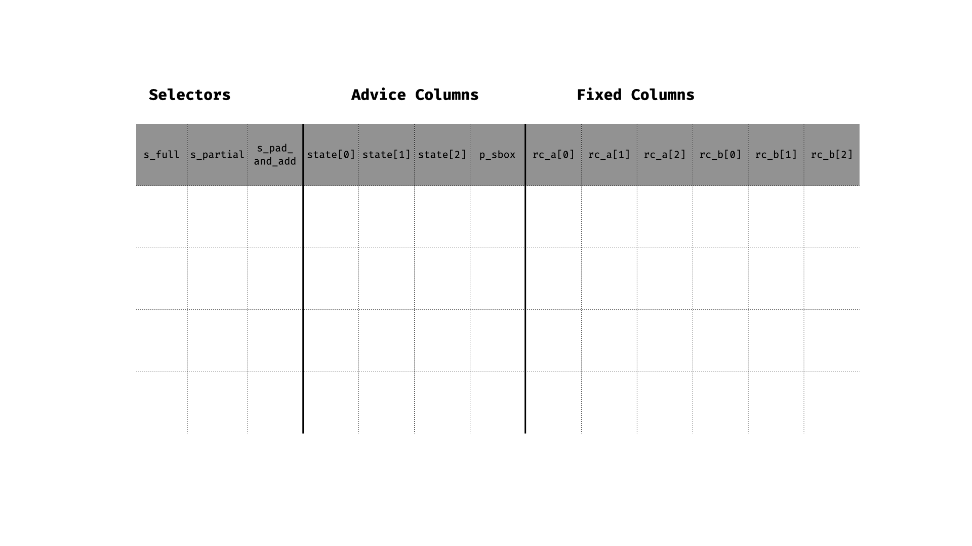
The chip has three gates: 1. Full Round. 2. Partial Round. 3. Pad-and-Add.

The permute function applies the first half of the full rounds, processes the partial rounds (applying the gate for two rounds per assignment), and finishes with the rest of the full rounds.

Let’s start with the full round. For each state element $\{0,1,2\}$, the following constraint is applied:

state[i]::next = (state[0]::cur + rc_a[0]::cur)^5 * m_reg[i][0] +
                 (state[1]::cur + rc_a[1]::cur)^5 * m_reg[i][1] +
                 (state[2]::cur + rc_a[2]::cur)^5 * m_reg[i][2]

This enforces that: 1. Round constants are added to each element. 2. The S-box ($x^5$) is applied to all elements. 3. MDS matrix multiplication is applied correctly. 4. The result matches the next row’s values.

The selector for this gate is enabled in the full_round function. Additionally, the assignment of constant values to the fixed column is handled by the round function.

Next, let’s proceed to the partial round gate, which is the most complex gate in the Pow5Chip. In this gate, two partial rounds are processed, where the S-box is applied only to the first state element. We can break this gate into three constraints.

S-box Constraint for Round A

The S-box for the first element during round A is constrained as:

(state[0]::cur + rc_a[0])^5 - partial_sbox::cur = 0

State After Round A: Closure Definitions

To define constraints for: 1. The second S-box for the first element combined with MDS multiplication. 2. Linear constraints for the other two states $\{1,2\}$ (addition of constants and MDS for both rounds).

We introduce the following closures:

1. mid(idx): Represents the state after round A:

mid(idx) = partial_sbox * m_reg[idx][0] +              // First element (after S-box)
           (state[1]::cur + rc_a[1]) * m_reg[idx][1] + // Second element (linear)
           (state[2]::cur + rc_a[2]) * m_reg[idx][2]   // Third element (linear)

2. next(idx): Computes the pre-MDS value for position idx:

next(idx) = state[0]::next * m_inv[idx][0] +
            state[1]::next * m_inv[idx][1] +
            state[2]::next * m_inv[idx][2]

Here’s why:

After both rounds, we have values in the next row $[x,y,z]$ produced by MDS multiplication:

Thus:

Constraints for Round B

1. S-box Constraint for the First Element: The second S-box, including MDS multiplication for round B, is constrained as:

(mid(0) + rc_b[0])^5 - next(0) = 0

2. Linear Constraints for Other Elements: The constraints for the second and third state elements are:

mid(1) + rc_b[1] - next(1) = 0
mid(2) + rc_b[2] - next(2) = 0

These constraints enforce: 1. Round A: S-box applied only to the first element, followed by MDS multiplication. 2. Round B: S-box applied only to the first element, followed by MDS multiplication.

Pad-and-Add Gate

Lastly, the pad-and-add gate handles absorption of inputs into the state. The table structure is as follows:

The constraints for updating the rate portion of the state are:

state[idx]::prev + state[idx]::cur - state[idx]::next = 0

// Equivalent to:
next_0 = prev_0 + input_0
next_1 = prev_1 + input_1

Constraints for the Capacity Element

The capacity element remains unchanged:

state[RATE]::prev - state[RATE]::next = 0

// Equivalent to:
next_2 = prev_2  // Capacity remains unchanged

This gate enforces that: 1. The rate portion elements are correctly updated with inputs. 2. The capacity element remains unchanged.

This gate is used in the add_input function.

Implementation Considerations

The Poseidon implementation in the Midnight circuits was designed to be parameterized, introducing an extra layer of abstraction in some parts of the code. However, the current implementation is specifically designed and tested to work with the three supported curves, with the WIDTH parameter set to 3 and the RATE set to 2.

If these parameters are modified, the implementation might fail to work correctly or even become insecure. For example, the following line (poseidon_gadget.rs:181) would be incorrect when RATE=1:

state.squeeze_position = 1

To ensure correctness and generalization, it should instead be updated to:

state.squeeze_position = (state.squeeze_position + 1) % RATE

This adjustment ensures compatibility with different RATE values and avoids potential implementation errors.

Sha256

Midnight implements the SHA-256 hash function in hash/sha256. Most of it is adapted from zcash halo2 lib. The Midnight implementation completes the implementation from the zcash (e.g., implementing the padding function). The main difference is that Midnight uses a smaller lookup table (called table11) that has about $2^{11}$ (instead of $2^{16}$) rows.

The SHA-256 works in several stages: padding, message scheduling, and compression. During padding, the input message is appended with a 1 bit, followed by enough 0 bits and a 64-bit representation of the message length to make its size a multiple of 512 bits. Next, the padded message is divided into 512-bit blocks, and each block undergoes message scheduling, where 64 words (each 32 bits) are generated. These words are derived from the block’s data and earlier words using bitwise operations and modular arithmetic. Finally, the compression stage processes each word through a series of rounds, using a state of eight 32-bit variables initialized to specific constants. Each round applies mathematical operations, mixing the input data with the current state until a final hash value is produced by combining the updated state variables.

The SHA-256 involves many bitwise operations, which are inefficient in modulo arithmetic. The circuit uses a “spread” technique to speed up the computation.

Spread

The spread operation maps an n-bit value to a 2n-bit value interleaved with zero bits. For example, given a 4-bit value a = 1011, the spread value a is 01_00_01_01.

The spread value is useful in transforming some bitwise operations into field element operations. For instance, in some functions of SHA-256, it is necessary to compute the bitwise xor of a and b: c = a xor b. We can transform this by spreading the value a and b to get a' and b'. Then calculate c' = a' + b, where the + here represents the modulo addition.

For example, let a = 1011 and b = 0110, then we should have c = a xor b = 1101. Using the spread values, we have a' = 01_00_01_01 and b' = 00_01_01_00. Then c' = a' + b' = 01_01_10_01. To get c, we need to extract the even bits (starting at 0 from right to left), which is exactly 1101. In this example, the spread value has an odd bit of zero as a “buffer” to hold the possible carry from an even bit.

The circuit uses a witness-and-check method to extract the even bits of c. It will witness two 4-bit values c_even and c_odd and enforce that c' = spread(c_even) + 2*spread(c_odd). Then, we will have c = c_even. With the example above, we will have c_even = 1101 and c_odd = 0010, and c_even is what we want.

The question then arises: How can we efficiently compute a value’s spread? The answer is to use a lookup table, as described below.

Spread Lookup Table

The circuit builds a static table with the original and corresponding spread values. Whenever it’s needed to do a spread, the circuit just performs a lookup into the table and gets the result.

Below is an example of the table:

The t_tag column marks the bit length of the value and ensures tables of different bit lengths are independent. The t_dense column is for the original value, and the t_spread is for the spread value.

Table 16 has about $2^{16}$ rows and supports 16-bit dense value lookup. In the with_lookup function, it assigns tag, dense, and spread into one row, forcing that row to exist in the lookup table. As the tag column is an advice column, the tag value needs to be range-checked to constrain the length of the dense value.

Table 11 has about $2^{11}$ rows and supports 11-bit dense value lookup. This efficiently reduces the row count in the table. To get the spread of a larger value, it will need to split the value into two pieces that are within 11-bit, do the lookup separately, and combine the spread pieces into one spread value. For example, in order to spread a 13-bit value, it will split it (decomposition.rs:244) to 10-bit and 3-bit pieces and then do the lookup. As in Table 11, the tag column is a fixed column; the tag value doesn’t need an extra range check.

Implementation of SHA-256

In the following, we describe the implementation of SHA-256 using the Table 16 spread table. The main differences between Table 16 and Table 11 have been described previously. In the implementation, the logic of Table 11 is implemented in the file src/hash/sha256/table11/decomposition.rs. Furthermore, in Table 11 we don’t require range checks in the tag column as it is a fixed column, and the checks of the validity of dense/spread are being saved in a postponed vector and checked later on.

Table 16 Tags

As already mentioned, Table 16 uses tags to range-check the number of bits for a dense value. The following code demonstrates the ranges supported and their respective tags.

pub fn get_tag(input: u16) -> u8 {
    let input = input as usize;
    if input < BITS_4 {
        0
    } else if input < BITS_7 {
        1
    } else if input < BITS_10 {
        2
    } else if input < BITS_11 {
        3
    } else if input < BITS_13 {
        4
    } else if input < BITS_14 {
        5
    } else {
        6
    }
}

If a value contains 11 bits, then the tag should be 0, 1, 2, or 3; thus, in the code, we will range-check it between 0 and 3.

Spec Mapping

Here are the columns used in the code renamed to match the spec. This will help us map the implementation to the actual specification.

a_0 = lookup_inputs.tag;
a_1 = lookup_inputs.dense;
a_2 = lookup_inputs.spread;
a_3 = extras[0];
a_4 = extras[1];
a_5 = message_schedule;
a_6 = extras[2];
a_7 = extras[3];
a_8 = extras[4];
a_9 = extras[5];

Message Schedule

Next, we will cover the message schedule process. When we call the compress function (table16.rs:239-240), we will provide as input some initial state and some inputs. The input is composed of AssignedBlockWords (32-bit words), and we have 16 such words (i.e., a 512-bit chunk).

The first step is to call the message_schedule.process function (message_schedule.rs:319). This function aims to create a 64-entry message array where w[0..15] are the 16 input words, and the rest are computed using the following loop.

for i from 16 to 63
    s0 := (w[i-15] rightrotate 7) xor (w[i-15] rightrotate 18) xor (w[i-15] rightshift  3)
    s1 := (w[i-2] rightrotate 17) xor (w[i-2] rightrotate 19) xor (w[i-2] rightshift 10)
    w[i] := w[i-16] + s0 + w[i-7] + s1

The code’s output will be an array of 64 MessageWords and an array of tuples containing the halves of each word (16-bit low and high parts). Let’s proceed to understand how those rows will be assigned and constrained. Firstly, we need to understand how the region of the message schedule is split. The implementation (schedule_util.rs:12-55) specifies how to split the region into subregions. In summary, we have the following subregions:

• Subregion 0: Handles $W_0$ (first word)
  • Uses DECOMPOSE_0_ROWS (2 rows)
• Subregion 1: Handles $W_1$ to $W_{13}$
  • Each word needs DECOMPOSE_1_ROWS + SIGMA_0_V1_ROWS (6 rows)
• Subregion 2: Handles $W_{14}$ to $W_{48}$
  • Each word needs DECOMPOSE_2_ROWS + SIGMA_0_V2_ROWS + SIGMA_1_V2_ROWS (11 rows)
• Subregion 3: Handles $W_{49}$ to $W_{61}$
  • Each word needs DECOMPOSE_3_ROWS + SIGMA_1_V1_ROWS (6 rows)
• Subregion 4: Would handle $W_{62}$ to $W_{63}$
  • Each word needs DECOMPOSE_0_ROWS (2 rows)

In the process function, we first enable (message_schedule.rs:339-371) all the appropriate gates based on the above separation. The s_decompose_0 gate is enabled for every word, and then, for each region, we enable the extra gates we need. For example, for subregion 2 (words 14 to 49), we will enable s_decompose_2, s_lower_sigma_0_v2, s_lower_sigma_1_v2, and s_word. Before explaining the gates, let’s explain how we perform the assignments and why we have split subregions this way.

Note: In the tables below that we demonstrate how cells are assigned and constraints are applied, we use the follow rules:

• Red cells represent cells used by the first gate.
• Green cells represent cells used by the second gate.
• Blue cells represent cells used by the third gate.
• Yellow cells represent cells used by the fourth gate.
• White cells represent cells that are not used by any gate but were assigned by one of the functions that enabled any of the gates that are involved.
• Grey cells represent cells that are assigned and used by functions/gates that were not described in the description of the specific section.

Assign the First 16 Words

The first step (message_schedule.rs:374-378) is to assign the first 16 words and also split them into halves. To do so, we use the function assign_word_and_halves that will get the row of the current word and the word value and will assign w_lo to a3, w_hi to a4, and word to a5. Note that the values that were assigned are out-of-circuit. Therefore, we have to check these assignments against the original inputs (e.g., table16.rs:267). The s_decompose_0 gate (schedule_gates.rs:41-50) will also be responsible for checking that the decomposition of each word happened correctly. The following table depicts the row for the s_decompose_0 gate.

Subregion 1 ($W_1$ to $W_{14}$)

Next is subregion 1. This subregion is required to decompose words and compute ${\sigma }_0$ values for the words from 1 to 14. The next subregion will handle the other words and computation of ${\sigma }_0$. We need this subregion because this is the only operation we apply in words $W_1$ to $W_{14}$. The function assign_subregion1 (subregion1.rs:87) will first decompose a word into four pieces: a (3-bit), b (4-bit), c (11-bit), and d (14-bit), according to the spec. For a and b, we will keep their dense form; for c and d, we will keep their spread form. Specifically, decompose_subregion1_word (subregion1.rs:113) assigns a to column a3 / row + 1 (from the current row word), b to column a4 / row + 1. Then, it will look up c into a1 (tag) / a2 (dense) / a3 (spread) in row + 1 and d in row.

The lower_sigma_0 function (subregion1.rs:171) will take as input the index of the word, a, b, spread_c, and spread_d. It will skip three rows. It first copies a into a5 in row + 1 and witnesses its spread value into a6 / row + 1. Then it copies b into a6 in the current row, split it into b_lo (assigned into a3 / row - 1) and b_hi (assigned into a5 / row - 1) and witness its spread values into a4 / row - 1 and a6 / row - 1. Next, it copies spread_c into a4 in the current row and spread_d into a5 in the same row. Then, it computes r using xor_lower_sigma_0 (subregion1.rs:47) which is basically the output of the ${\sigma }_0$ function. Finally, it splits r into $R_0^{even}$, $R_0^{odd}$, $R_1^{even}$, $R_1^{odd}$ and uses assign_sigma_outputs (table16.rs:463) that calls assign_spread_outputs (table16.rs:411), which will do the following 4 lookups into columns a1, a2, and a3:

• lookup $R_0^{even}$ in row - 1
• lookup $R_0^{odd}$ in row
• lookup $R_1^{even}$ in row + 1
• lookup $R_1^{odd}$ in row + 2

Finally, it copies the spread format of $R_1^{odd}$ in column a3 in the current row and returns r_0 and r_1 in their dense form. Note that lower_sigma_0 returns $R_0^{even}$ and $R_1^{even}$ in dense form.

The following gates are enforced in this subregion (on top of s_decompose_0):

• s_decompose_1 (schedule_gates.rs:54) is used to check the correct decomposition of a word into pieces a, b, c, and d. Note that a and b are not range-checked as they have already been range-checked in s_lower_sigma_0.
• s_lower_sigma_0 (schedule_gates.rs:156) first range-checks and checks the spreads of the variables a and b. Then, it checks if the spread witness values (spread values for r0_even, r0_odd, r1_even, and r1_odd that compose the output of lower_sigma_0) equals $(X⋙7)\oplus (X⋘14)\oplus (X\gg 3)$, where $X$ is our word and we follow the equations described in the spec. Note that we provide a complete explanation of one of a Sigma functions later in this document. The others follow similar techniques and logic.

The table for the first row will look like this:

Subregion 2 ($W_{14}$ to $W_{49}$ – produces $W_{16}$ to $W_{50}$)

Recall that from subregion 1, we have computed the ${\sigma }_0$ values for the words from 1 to 14, and we have returned $R_0^{even}$ and $R_1^{even}$ in dense form. In the function assign_subregion2 (subregion2.rs:164), we pass those ${\sigma }_0$ values, we assign the new words from $W_{16}$ to $W_{49}$ along with their decomposed halves, we make all the assignments and add all the constraints required, and finally, we return the output of sigma_0_v2 on $W_{36}$ to $W_{49}$ to use them in subregion 3.

In assign_subregion2, the closure to compute a new word is: $W_i={\sigma }_1(W_{i-2})+W_{i-7}+{\sigma }_0(W_{i-15})+W_{i-16}$, e.g., $W_{16}={\sigma }_1(W_{14})+W_9+{\sigma }_0(W_1)+W_0$. To compute the new words, we are going to use the following:

• sigma_0(W_[1..14]) (from subregion 1) will be used to get the new W_[16..29]
• sigma_0_v2(W_[14..36]) will be used to get the new W_[29..51]
• sigma_1_v2(W_[14..49]) will be used to get the W_[16..51]

The closure new_word (subregion2.rs:190) takes as input an index and sigma_0_output. This closure will create new words for index + 2 ($W_{i+2}$). For example, when we are at index 14 (i.e., word at index 14 – $W_{14}$), we will produce a new word for $W_{16}$. For the first 13 indexes, we are going to create new words. We will use the ${\sigma }_0$ values from subregion 1. Then, for each index, we will compute ${\sigma }_0$ that will be used to produce words at $W_{i+15}$ and ${\sigma }_1$ that will be used to produce $W_{i+2}$ (i.e., the word we are producing in the iteration). Note that for indexes 27..49, we will use ${\sigma }_0$, which was produced when looping through indexes 14..27.

The function decompose_word (subregion2.rs:299) is responsible for decomposing a word similar to the previous decompose functions. Specifically, it will assign the following cells:

• a will be assigned in column a3 / row - 1
• b will be looked up at row + 1
• c will be assigned in column a4 / row - 1
• d will be looked up at the current row
• e will be assigned in a3 / row + 1
• f will be assigned in a4 / row + 1
• g will be looked up at row - 1

Next, lower_sigma_0_v2 (subregion2.rs:426) computes ${\sigma }_0$ values for the current word ($W_i$) – that will be used in a next iteration. This function works at row + 3 from the current row. First, it calls assign_lower_sigma_v2_pieces (subregion2.rs:363), which is responsible for copying and constraining the pieces of the decomposed word to use them in either lower_sigma_0_v2 or lower_sigma_1_v2. This will lead to the following:

• a will be copied into a3 / row + 1
• spread_a will be assigned into a4 / row + 1
• b will be copied into a6 / row
• b_lo will be assigned into a3 / row - 1
• spread_b_lo will be assigned into a4 / row - 1
• b_hi will be assigned into a5 / row - 1
• spread_b_hi will be assigned into a6 / row - 1
• c will be copied into a5 / row + 1
• spread_c will be assigned into a6 / row + 1
• spread_d will be copied into a4 / row
• e will be copied into a7 / row
• f will be copied into a7 / row + 1
• spread_g will be copied into a5 / row

Then, it will compute the output of ${\sigma }_0^{v2}$ according to the spec (r), calculate $R_0^{even}$, $R_0^{odd}$, $R_1^{even}$, $R_1^{odd}$, and will perform the following operations by using assign_sigma_outputs:

• It will lookup $R_0^{even}$ in row - 1
• It will lookup $R_0^{odd}$ in row
• It will lookup $R_1^{even}$ in row + 1
• It will lookup $R_1^{odd}$ in row + 2
• It will copy $\text{spread}(R_1^{odd})$ in a3 / row

The exact same process will be followed for ${\sigma }_1^{v2}$ by calling lower_sigma_1_v2. You can see the resulting table below.

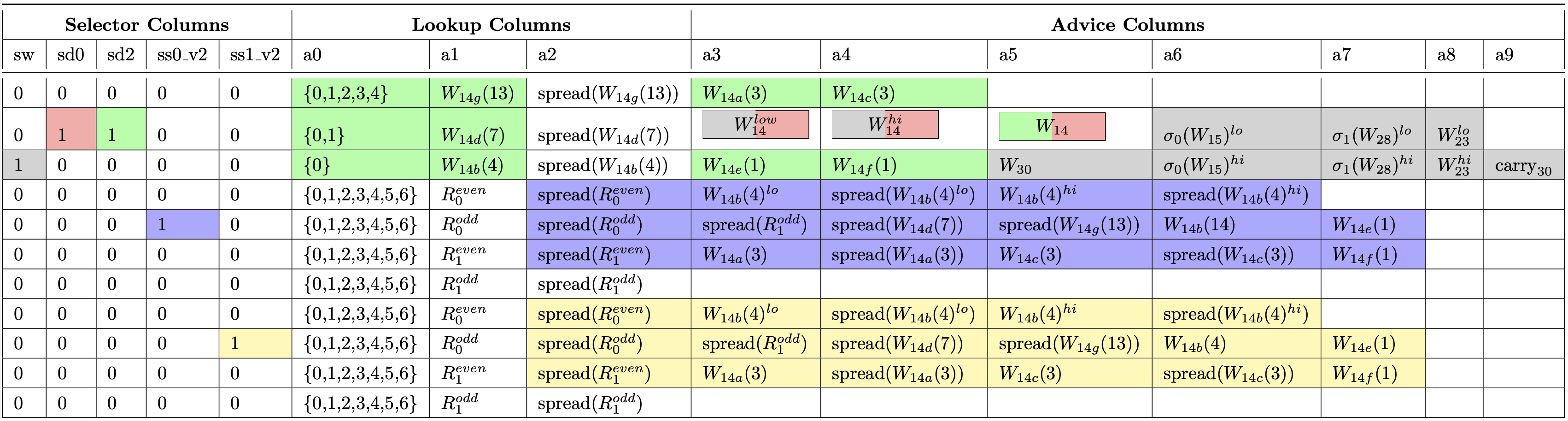
Next, it will compute the new word and its carry, and it will witness it at:

• $W_{ni}$ in column a5 at the row of $W_{ni-16}$ + 1
  • E.g., $W_{16}$ in column a5 at the row of $W_0$ + 1
• ${\text{carry}}_{ni}$ in column a9 at the row of $W_{ni-16}$ + 1
  • E.g., ${\text{carry}}_{16}$ in column a9 at the row of $W_0$ + 1

Finally, it uses assign_word_and_halves (schedule_util.rs:154). This function will assign the new word and its halves in the ni. Specifically:

• It will assign $W_{ni}^{lo}$ in column a3 of the row of the new word.
• It will assign $W_{ni}^{hi}$ in column a4 of the row of the new word.
• It will assign $W_{ni}$ in column a5 of the row of the new word.

Note that for words $W_0$ to $W_{16}$, this has happened in the process function (message_schedule.rs:374) of message schedule.

The following gates are enforced in this subregion (on top of s_decompose_0):

• s_decompose_2 (schedule_gates.rs:82) is used to check the correct decomposition of a word to a, b, c, d, e, f, and g pieces. Note that a and c are range-checked in s_lower_sigma_0_v2 and s_lower_sigma_1_v2.
• s_lower_sigma_0_v2 (schedule_gates.rs:274) first range-checks a, c, b_lo, and b_hiwhile also checking their spread values. Next, it checks if the spread values we have witnessed in r0_even, r0_odd, r1_even, and r1_odd equal the expected result according to the spec.
• s_lower_sigma_1_v2 (schedule_gates.rs:340) does pretty much the same as s_lower_sigma_0_v2 but for ${\sigma }_1$.
• The s_word gate (schedule_gates.rs:13) checks if the computed words for $W_{16}$ to $W_{63}$ are correct according to the spec (i.e., $W_i={\sigma }_1(W_{i-2})\oplus W_{i-7}\oplus {\sigma }_0(W_{i-15})\oplus W_{i-16}$) – The cells for new word are depicted with gray color in the figure and are from index 30.

Subregion 3 ($W_{49}$ to $W_{62}$ – produces $W_{51}$ to $W_{63}$)

The logic for assign_subregion3 (subregion3.rs:86) is almost the same as for assign_subregion2. This function takes as input all the required ${\sigma }_0$ values. In the following, we will cover the differences with subregion 2.

Firstly, the decompose_subregion3_word (subregion3.rs:202) follows a logic similar to decompose_subregion1_word, but for different pieces. Next, the logic of lower_sigma_1 (subregion3.rs:247) closely follows the logic of lower_sigma_0, but implements a different function. The rest of the code closely follows the logic of the assign_subregion2 function.

The following gates are enforced in this subregion on top of s_decompose_0:

• s_decompose_3 (schedule_gates.rs:121) similar to s_decompose_1.
• s_lower_sigma_1 (schedule_gates.rs:209), similar to s_lower_sigma_0, but constraints the ${\sigma }_1$ function. Additionally, it range-checks and enforces the proper spread for b_lo, b_mid, b_hi, c, and checks b.

For reference, here is the table for $W_{49}$:

The Sigma Function

The sigma function is used both in the message schedule and compression process. Specifically, lower Sigma (${\sigma }_0$ and ${\sigma }_1$) are used in the message schedule, and upper Sigma (${\Sigma }_0$ and ${\Sigma }_1$) are used in compression. As these sigma functions work in the same way (only have a difference in the shifting number), here we only introduce ${\sigma }_0$. By definition:

Where $X$ is the 32-bit word. It is equivalent to

To perform the shifting, we can split $X$ into smaller pieces. To perform $X⋙7$, we can split $X$ at the 7-th bit and get 7-bit number $x_1$ and 25-bit number $x_2$. Then we have $(X⋙7)=x_1+2^7{x}_2$. Similarly, for $X⋘14$, we can split $X$ into 14-bit numbers and 18-bit numbers. For $X\gg 3$, we can split $X$ into 3-bit numbers and 29-bit numbers. Splitting three times together we will have 4 pieces: $(a,b,c,d)$ of lengths $(3,4,11,14)$. The figure below is taken from the halo2 book:

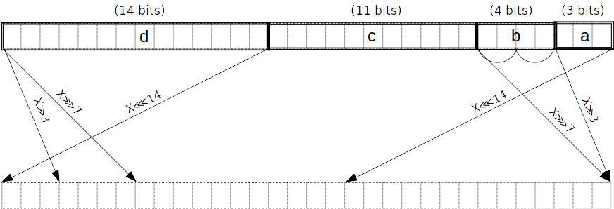
Then we have

The last step is to compute the xor of the three shifted values. The code takes the spread form of $X$ and splits that into spread pieces: $(a^{\prime },b^{\prime },c^{\prime },d^{\prime })$. Then get the spread form of shifted values and perform the xor operation by adding these values: $spread(X⋙7)+spread(X⋘14)+spread(X\gg 3)$. Finally, it extracts the dense value from the spread result in the way introduced before

Compression

In this section, we will review the spec and code for the compression phase of Sha256. Thus, compression has two phases.

Initialize

First, we need to initialize the state with the initialization vector (iv). That is the role of the initialization_vector function (table16.rs:217). This function will then call initialize_with_iv (compression.rs:937) that will assign a new region for the initial state, will do the assignments by calling the initialize_iv function (subregion_initial.rs:16), and will return a variable containing the state that is composed of StateWords (compression.rs:467).

Decompose Variables

The initialize_iv function is responsible for decomposing and assigning into the table the initial values for the variables A, B, C, E, F, G, and assigning the halves (low and high) of the dense format of the variables D and H. A neat reference for visualizing the result of this function is the table Initial round from the specification. This table has 31 rows. In row 0, we decompose variable E. Note that in the code, we select the rows by using the get_round_row function (compression_util.rs:100) and adding lines based on the variable we are handling. Now, to decompose variable E, we are calling the function decompose_iv_e (compression_util.rs:390). This function will first load the value of IV for E, then it will select the proper row, and then it will use the assign_word_halves_fixed function (compression_util.rs:1064). This function will break the 32-bit word into two 16-bit variables (low and high), then it will compute the spread format for both of them, and it will assign to the cells at column a7 and a8 in the current row the dense and spread for the low part, and in the next row in the same columns for the high part. After calling assign_word_halves_fixed, we call the decompose_efgh function (compression_util.rs:399) that will enable the s_decompose_efgh gate (compression_gates.rs:87), do all the proper assignments and lookups, and will return an EfghVar (compression.rs:179). This will break the variable into (6,5,14,7) bit-chunks, respectively. The first part is split into 3 (low) and 3 (high), and the second into 2 (low) and 3 (high).

According to the docs, we need to break the variable into those pieces because:

• In Σ_1(E), we need E to be split into pieces (a,b,c,d) of lengths (6,5,14,7) bits, respectively (counting from the little end), as well as their spread forms.
• Ch(E,F,G) requires the bits of each input to be in spread form. For E, we can reuse the pieces from Σ_1(E). Since F and G are assigned from E and F, respectively, in each round, we also have the same pieces in earlier rows. We align the columns to make it efficient to copy-constrain these forms where they are needed.

We will see why this is the case later on.

The s_decompose_efgh gate is responsible for (1) range-checking the inputs, (2) checking if the spread value is correct, (3) checking for both the dense and spread formats if the sum of the pieces is equal to the dense and spread form of the original word. To do so, for a_lo/a_hi/b_low/b_hi, it uses three_bit_spread_and_range (gates.rs:99-100) and two_bit_spread_and_range (gates.rs:73) which first checks if dense is in the correct range and then if the provided dense is the correct one for the spread. For c and d, we have performed two lookups (compression_util.rs:337) in decompose_efgh. This means that, indeed there exists a row in the lookup table that contains tag,dense,spread. What is missing here is that we use an appropriate tag to enforce the range check. This happens in the gate (compression_gates.rs:126). For c, we check that the tag is in {0,1,2,3,4,5} as a 14-bit value; for d, we check that the tag is in {0,1} as a 7-bit value. The resulting table for decompose_iv_e will look like this:

Next, we call decompose_iv_f (subregion_initial.rs:167) and decompose_iv_g (subregion_initial.rs:195). Those functions are similar to decompose_iv_e, but they chose other rows and also return a simple RoundWord composed of dense and spread halves, instead of an EfghVar. Finally, for variable h, we just use assign_word_halves_dense_fixed to assign the low and high halves of its dense form in column a7 in rows 10 and 11 of the region.

Similar logic is followed for variables A, B, C, and D. Note that AbcdVar (compression.rs:88) is split accordingly:

• In Σ_0(A), we need A to be split into pieces (a,b,c,d) of lengths (2,11,9,10) bits respectively (counting from the little end), as well as their spread forms. Note that c is split into three parts of 3 bits each (i.e., lo, mid, hi).
• Maj(A,B,C) requires the bits of each input to be in spread form. For A, we can reuse the pieces from Σ_0(A). Since B and C are assigned from A and B, respectively, in each round. We, therefore, also have the same pieces in earlier rows. We align the columns to make it efficient to copy-constrain these forms where they are needed.

With that, we have finished the initialize_iv function, initialized the state with the original values, and assigned the values to the proper cells. The logic for initialize_state (subregion_initial.rs:61) is pretty much the same, with the addition that this function consumes a previous state. Hence, equality constraints are applied between the dense values from the cells of the previous state and the values in the newly assigned cells. Specifically, what it changes is that the decompose_{a,b,c,d,e,f,g,h}_iv functions are using assign_word_halves_fixed, whereas decompose_{a,b,c,d,e,f,g,h} are using assign_word_halves and then constrain the cell that it gets the value from to equal the cell that assigns the values to (the dense halves). Note that for decompose_{a,e} this is required only in the first round because later it is enforced in the code (subregion_main.rs:87).

Compress

The compress function (compression.rs:972) gets as input some initialized state and a message schedule (i.e., 64 words in halves). The function will first apply the initialized state, loop over the 64 words, and apply a compression round for each one. In the end, the resulting state is the output that we can then digest.

The main logic is implemented in the assign_round function (subregion_main.rs:13) that takes as input the round number, the previous state that we require in the last round, the current state (in the first round, it is the same as the previous state), and the halves of the word we are processing in this round. The function will return the new state that will be used in the next round as the state input.

Let’s now analyze what is happening when assigning a round. The following operations are being applied.

${\Sigma }_1$

First, the ${\Sigma }_1$ function is applied that inputs the pieces of e from the state (look at decompose_efgh), the round index, and computes sigma_1. The assign_upper_sigma_1 function (compression_util.rs:480) does the following:

• It copies $\text{spread}{E}_0{a}^{lo}(6)$ into column a3 / row + 1
• It copies $\text{spread}{E}_0{a}^{hi}(6)$ into column a4 / row + 1
• It copies $\text{spread}{E}_0{b}^{lo}(5)$ into column a3 / row - 1
• It copies $\text{spread}{E}_0{b}^{hi}(5)$ into column a4 / row - 1
• It copies $\text{spread}{E}_0{c}^{hi}(14)$ into column a5 / row
• It copies $\text{spread}{E}_0{d}^{hi}(7)$ into column a4 / row

Next, it computes r by following the spec definition for ${\Sigma }_1$, and it calculates $R_0^{even}$, $R_0^{odd}$, $R_1^{even}$, $R_1^{odd}$. Then, it calls assign_sigma_outputs that calls assign_spread_outputs (table16.rs:411) and performs the following operations:

• It will lookup $R_0^{even}$ in row - 1
• It will lookup $R_0^{odd}$ in row
• It will lookup $R_1^{even}$ in row + 1
• It will lookup $R_1^{odd}$ in row + 2
• It will copy $\text{spread}(R_1^{odd})$ in a3 / row

Then, it will finally return $R_0^{even}$ and $R_1^{even}$ in dense form. On top of that, for ${\Sigma }_1$, the s_upper_sigma_1 gate (compression_gates.rs:201) will be enabled. This gate checks that the spread witnessed values of r equals ${\Sigma }_1$ according to the spec. This assign function will result in the following table:

$Ch$ function

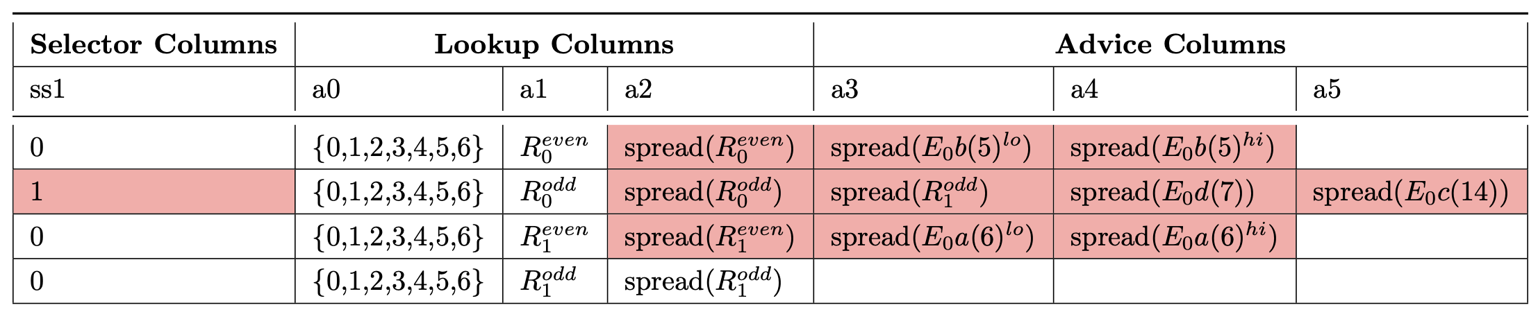
The $Ch$ function is defined as follows: $Ch(E,F,G)=(E\wedge F)\oplus (\neg E\wedge G)$. We refer the interested reader to the spec for understanding how we can implement $Ch$ efficiently. Here, we are going to discuss the implementation. So, first of all we have all $E,F,G$ in their spread form. To implement that operation we want to compute $Ch=P=\text{spread}(E)+\text{spread}(F)$ and $C{h}_{neg}=Q=(evens-E)+G=((\text{spread}(2^{32}-1)-\text{spread}(E))+\text{spread}(G)$.

The assign_ch function (compression_util.rs:565) performs the computation and the assignments for the first part (i.e., $P$). Specifically, it does the following:

• It copies $\text{spread}(E^{lo})$ into column a3 / row - 1
• It copies $\text{spread}(E^{hi})$ into column a4 / row - 1
• It copies $\text{spread}(F^{lo})$ into column a3 / row + 1
• It copies $\text{spread}(F^{hi})$ into column a4 / row + 1

Next, it computes p by following the spec definition (i.e., adding the spread halves of $E$ and $F$), and it calculates $P_0^{even}$, $P_0^{odd}$, $P_1^{even}$, $P_1^{odd}$. Then, it calls assign_ch_outputs which in turn calls assign_spread_outputs (it performs all the necessary lookups and assigns $P_1^{odd}$) and returns the tuple ($P_0^{odd}$, $P_1^{odd}$). Additionally, the gate s_ch (compression_gates.rs:244) is enabled, which checks if the witnessed values have been computed correctly according to the spec.

The assign_ch_neg function (compression_util.rs:611) follows a similar logic. The main addition is that the implementation computes and assigns $\text{spread}(E_{neg}^{lo})$ and $\text{spread}(E_{neg}^{lo})$ (compression_util.rs:642-668). Accordingly, in the respective gate, we have an additional check (compression_gates.rs:287).

${\Sigma }_0$

We skip the explanation of ${\Sigma }_0$ as it is almost identical to ${\Sigma }_1$.

Maj function

The Maj function is defined as follows: $Maj(A,B,C)=(A\wedge B)\oplus (A\wedge C)\oplus (B\wedge C)$. As we already have $A,B,C$ in spread form, we can compute $M=\text{spread}(A)+\text{spread}(B)+\text{spread}(C)$, then we witness the $M_i^{even}$ and $M_i^{odd}$ bits of the halves of $M$, and the result of $Maj$ is $M_i^{odd}$. To make it work correctly, we also need a gate to constrain the witnessed values.

Let’s see how this function is implemented. Firstly, we use the assign_maj function (compression_util.rs:714) which does the following:

• It copies $\text{spread}(A^{lo})$ into column a4 / row - 1
• It copies $\text{spread}(A^{hi})$ into column a5 / row - 1
• It copies $\text{spread}(B^{lo})$ into column a4 / row
• It copies $\text{spread}(B^{hi})$ into column a5 / row
• It copies $\text{spread}(C^{lo})$ into column a4 / row + 1
• It copies $\text{spread}(C^{hi})$ into column a5 / row + 1

Next, it computes m by following the spec definition (i.e., adding the spread halves of $A$, $B$, and $C$), and it calculates $M_0^{even}$, $M_0^{odd}$, $M_1^{even}$, $M_1^{odd}$. Then, it calls assign_maj_outputs, which in turn calls assign_spread_outputs (it performs all the necessary lookups and assigns $M_1^{odd}$). Lastly, it returns the tuple ($M_0^{odd}$, $M_1^{odd}$). Additionally, the gate s_maj (compression_gates.rs:312) is enabled which checks if the witnessed maj values have been computed correctly according to the spec.

$H^{\prime }$

In a round $i$, we compute $H^{\prime }$ as $H+Ch(A,B,C)+{\Sigma }_1(E)+K_i+W_i$. This logic is implemented in function assign_h_prime (compression_util.rs:772) that takes as input the round_idx round number, h (from the state), ch (computed by assign_ch), ch_neg (computed by assign_ch_neg), sigma_1 (as computed by assign_upper_sigma_1), ROUND_CONSTANT[round_idx] ($K_i$), and schedule_word ($W_i$). The function then performs the following operations:

• It copies $H^{lo}$ into column a7 / row - 1
• It copies $H^{hi}$ into column a7 / row
• It copies ${\Sigma }_1^{lo}$ into column a4 / row
• It copies ${\Sigma }_1^{hi}$ into column a5 / row
• It assigns $K^{lo}$ into column a6 / row - 1
• It assigns $K^{hi}$ into column a6 / row
• It copies $W^{lo}$ into column a8 / row - 1
• It copies $W^{hi}$ into column a8 / row
• It copies $C{h}^{hi}$ into column a6 / row + 1
• It copies $C{h}_{neg}^{lo}$ into column a5 / row - 1
• It copies $C{h}_{neg}^{hi}$ into column a5 / row + 1
• It computes h_prime_low, h_prime_high, and h_prime_carry
• It assigns $H_{carry}^{\prime }$ into column a9 / row + 1
• It assigns $H^{\prime lo}$ into column a7 / row + 1
• It assigns $H^{\prime hi}$ into column a8 / row + 1

Finally, it returns (h_prime_low, h_prime_high). Additionally, the s_h_prime gate (compression_gates.rs:339) performs a check to verify that h_prime_low, h_prime_high, and h_prime_carry have been computed correctly. The following table demonstrates the cells assigned by assign_h_prime.

Note that in this region, we also apply assign_ch and enforce the constraints of the gate s_ch. Hence, all the cells colored green are the cells used by s_ch gate, whereas the cells colored red are used by s_h_prime gate. Finally, the white cells in columns a0 and a1 are assigned by the lookups in assign_ch along with the cell at the last row in column a2 (is copied at row 2 / column a3) while the cells at the last row in columns a5 and a6 are assigned and used by $E_{new}$ (gray color).

$E_{new}$

To compute $E_{new}$ we need to do $H^{\prime }+D$. The function assign_e_new (compression_util.rs:906) is responsible for performing that operation. It does the following:

• It copies $D^{lo}$ into column a7 / row
• It copies $D^{hi}$ into column a7 / row + 1
• It computes e_new (dense form) and e_new_carry
• It assigns $E_{new}^{lo}$ into column a8 / row
• It assigns $E_{new}^{hi}$ into column a8 / row + 1
• It assigns $E_{carry}$ into column a9 / row + 1

Additionally, it applies the gate s_e_new (compression_gates.rs:418) which checks if e_new has been computed correctly.

Note that only the red cells are being used by the gate s_e_new. The gray cells have been assigned by other parts of the code and used by other gates.

$A_{new}$

To compute $A_{new}$ we need to do $H^{\prime }+Maj(A,B,C)+{\Sigma }_0(A)$. The function assign_a_new (compression_util.rs:938) is responsible for performing that operation. It does the following:

• It copies $Ma{j}^{hi}$ into column a3 / row - 1
• It copies ${\Sigma }_0^{lo}$ into column a6 / row
• It copies ${\Sigma }_0^{hi}$ into column a7 / row + 1
• It copies $H^{\prime lo}$ into column a7 / row - 1
• It copies $H^{\prime hi}$ into column a8 / row - 1
• It computes a_new (dense form) and a_new_carry
• It assigns $A_{new}^{lo}$ into column a8 / row
• It assigns $A_{new}^{hi}$ into column a8 / row + 1
• It assigns $A_{carry}$ into column a9 / row

Additionally, it applies the gate s_a_new (compression_gates.rs:394) that checks if a_new has been computed correctly.

Note that in this region, we also apply assign_maj and enforce the constraints of the gate s_maj. Hence, all the cells colored green are the cells used by s_maj gate, whereas the cells colored red are used by s_a_new gate. Finally, the white cells in columns a0 and a1 are assigned by the lookups in assign_maj along with the cell at the last row in column a2 (copied at row 2 / column a3).

round_idx < 63 Case (Not the Last Round)

If we are not in the last round, we need to prepare the state for the next round. To do so, we copy a_new_dense and e_new_dense to the respective cell in the rows of the next round (subregion_main.rs:78). Furthermore, we also decompose in the rows of the new round by employing decompose_a and decompose_e. Finally, we create a new state and return it. The new state is composed of the following:

• A := a_new
• B := A
• C := B
• D := C
• E := e_new
• F := E
• G := F
• H := G

The Last Round

In the last round, we want to achieve the following state

• A := h0 + A
• B := h1 + B
• C := h2 + C
• D := h3 + D
• E := h4 + E
• F := h5 + F
• G := h6 + G
• H := h7 + h

Where h{0..7} are the initial values in the initial state at round 0. The implementation (subregion_main.rs:111) is responsible for that and will perform the following operations:

• It assigns $A_{new}^{lo}$ into column a3 / abcd_row
• It assigns $A_{new}^{hi}$ into column a4 / abcd_row
• It assigns $E_{new}^{lo}$ into column a3 / efgh_row
• It assigns $E_{new}^{hi}$ into column a4 / efgh_row

Then, for A to H, it will use the assign_state_addition function (compression_util.rs:873), that will take as input two terms and a row. For example, for A, term1 is h0 (prev_a.dense_halves – the dense halves of the initial A in round 0) and term2 is $A_{new}$ (dense halves). For B, term1 is h1 (prev_b.dense_halves) and term2 is A (a.dense_halves). The function performs the following operations:

• It assigns $ter{m}_1^{lo}$ into column a3 / row
• It assigns $ter{m}_1^{hi}$ into column a4 / row
• It assigns $ter{m}_2^{lo}$ into column a5 / row
• It assigns $ter{m}_2^{hi}$ into column a6 / row

It then computes the sum of the two terms into st_new and st_carry and does the following:

• It assigns $s{t}_{new}^{lo}$ into column a7 / row
• It assigns $s{t}_{new}^{hi}$ into column a8 / row
• It assigns $s{t}_{carry}$ into column 9 / row

Additionally, it enables the gate s_add_havles (compression_gates.rs:372), which checks if the addition was performed correctly. Lastly, the final state is added to a new state and returned to the compress function. The table below depicts the cells assigned by assign_state_addition and used by s_add_halves gate.

Digest

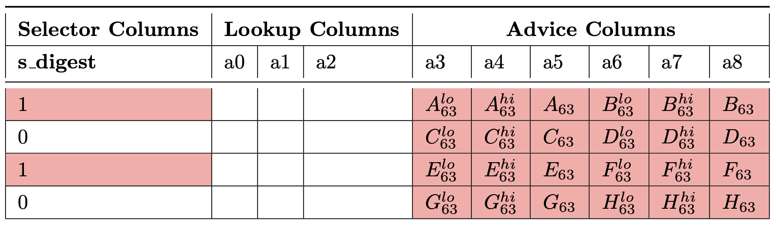
The last step of Sha256 is the digest step, which takes the state after the final round and converts it to the final digest. The main function that performs the digest is the assign_digest function (subregion_digest.rs:16) which takes as input some final state. This function performs the following operations:

• It copies $A^{lo}$ into column a3 / abcd_row
• It copies $A^{hi}$ into column a4 / abcd_row
• It computes $A$ (field element) and assigns it into column a5 / abcd_row
• It copies $B^{lo}$ into column a6 / abcd_row
• It copies $B^{hi}$ into column a7 / abcd_row
• It computes $B$ (field element) and assigns it into column a8 / abcd_row

It does the same for $C$ and $D$ but in row abcd_row + 1, and it performs the equivalent operations for $E,F,G,H$ but in rows efgh_row and efgh_row + 1. Moreover, it applies the s_digest gate (compression_gates.rs:440) in both abcd_row and efgh_row. This gate checks that the word computation was performed correctly. Finally, it returns the final words. The table below depicts the rows used for s_digest.

Issues in the Spec

Here, we report inconsistencies between the code and the specification or issues found in the specification. Note that this is not an exhaustive list, as most tables in the specification contain issues.

• In the initial and steady table in row 0, $F_{0}d(7)$ should be $E_{0}d(7)$. In the Message scheduling region part, in the table, in row 8, columns a3-a6, there are some values that are not described in the implementation or the spec.
• s_e_new is off by one row.
• Final digest table D values are switched by C values

Map

The MapGadget (src/map/map_gadget.rs) is an implementation of a key-value store using Merkle trees. In the Midnight protocol, this gadget serves the following functions:

• Implementing efficient key-value storage with ZK proofs.
• Proving membership in sets (see examples/membership.rs).

The key advantage of this implementation lies in its succinct representation through Merkle trees. Instead of proving statements about the entire map, proofs require only logarithmic-sized paths through the tree, making it both space- and computation-efficient for ZK circuits. At a high level, keys are represented as the path from the root to a leaf where the respective value is stored. The height of the tree is predefined as 128, which is a critical security parameter, as we will see.

Key Representation and Tree Traversal.

Given a field element $k$, its index is computed by hashing $k$, transforming it into bytes, and extracting the first 128 bits. This produces a bit string such as 1000101..., which is used to traverse the tree: move left for 0 and right for 1, starting from the root node. The state maintained for the Map is as follows:

struct State<F, H> {
    succinct_repr: AssignedNative<F>,  // The Merkle root representing the map
    map: Box<MapMt<F, H>>              // The underlying map structure
}

The succinct_repr corresponds to the Merkle root, providing a compact representation of the map. For example, consider a tree with height 2. Initially, all leaves are set to 0. Setting the key 0 to the value 1 would involve the following:

Map[0] = 1
hash(0) = 0x1234...
bits(0x1234...) = 0b10010001...
path[0] = [leaf_1_1, node_0, root]

This maps to a Merkle tree as shown below:

                 root Hash(node_0, node_1)
                /      \
               /        \
           node_0        node_1 Hash(leaf_1_0, leaf_1_1)
          /      \     /      \
         /        \   /        \
   leaf_0_0  leaf_0_1  leaf_1_0  leaf_1_1
        0         0         0         0

Here, path[0] contains the values needed to recompute the root, which must match the new succinct_repr. Verification logic is handled by the verify_path function:

fn verify_path(
    &self, 
    layouter: &mut impl Layouter<F>,
    key: &AssignedNative<F>,
    value: &AssignedNative<F>,
    proof: &[AssignedNative<F>; TREE_HEIGHT as usize]
) -> Result<(), Error> 
{
    // Compute path from key
    let zero = self.native_gadget.assign_fixed(layouter, F::ZERO)?;
    let path = self.hash_chip.hash(layouter, &[key.clone(), zero])?;
    let path_as_bits = self.native_gadget
        .assigned_to_le_bits(layouter, &path, None, true)?;

    // Reconstruct root from path
    let mut node: AssignedNative<F> = value.clone();
    for (is_right, sibling) in path_as_bits[..TREE_HEIGHT as usize]
        .iter()
        .zip(proof.iter()) 
    {
        // Determine left/right positioning
        let (left_sibling, right_sibling) = self
            .native_gadget
            .cond_swap(layouter, is_right, &node, sibling)?;

        // Hash to get parent
        node = self.hash_chip
            .hash(layouter, &[left_sibling, right_sibling])?;
    }

    // Verify computed root matches stored root
    self.native_gadget
        .assert_equal(layouter, &node, &self.state().succinct_repr)?;
    Ok(())
}

Insert and Get Operations.

If the verify_path operation passes, insertion and retrieval operations can be performed. For insertion: 1. Retrieve the path for the current value of the key and prove its correctness. 2. Update the state (in-circuit) to reflect the new root. 3. Prove the correctness of the new root using verify_path.

Security Considerations.

For a naive example with height 2, collisions are trivial to find. With a height of 128, as chosen in Midnight, the collision probability for any two keys is approximately $2^{-64}$. While this is sufficient for most use cases, it might not be adequate for applications requiring higher collision resistance.

ECC Native

The ecc/native implements twisted Edwards curve over native field in the format of $-x^2+y^2=1+d·x^2·y^2$ (i.e. with $a=-1$). On a twisted Edwards curve, the identity point has affine coordinates and the addition is complete. In EccChip the point is defined as x and y coordinates in native field.

/// A twisted Edwards curve point represented in affine (x, y) coordinates, the
/// identity represented as (0, 1).
#[derive(Clone, Debug)]
pub struct AssignedNativePoint<C: CircuitCurve> {
    x: AssignedNative<C::Base>,
    y: AssignedNative<C::Base>,
}

The scalar field element is represented as a vector of assigned bits (of native field) in little endian:

/// Scalars are represented as a vector of assigned bits in little endian.
#[derive(Clone, Debug)]
pub struct ScalarVar<C: CircuitCurve>(Vec<AssignedBit<C::Base>>);

The chip uses membership_gate to enforce a point is on-curve. That’s basically checking the equation of the curve.

Enforce P = (x, y) is on the curve, using columns:
---------------
|  x   |  y   |
---------------

We enforce:

 -x^2 + y^2 = 1 + d * x^2 * y^2

The assign function assigns a point from an off-circuit value. It first assigns a point and ensures it is on-curve via the membership_gate. Then multiply the point with cofactor to get the result. This ensures that the result point always lies in the correct subgroup although the result might not be identical to the input.

The chip uses two gates to perform point addition and multiplication. The double_gate gate enforces that Q(xq, yq) = [2]P(xp, yp):

Enforce Q = 2 * P, using columns:
-----------------------------
|  xp  |  yp  |  xq  |  yq  |
-----------------------------

The cond_add_gate enforces that R(xr, yr) = Q(xq, yq) + b * S(xs, ys) where b is 0 or 1:

Enforce R = Q + b * S, using columns:
-------------------------------------------------
|      |      |  xq  |  yq  |  xs  |  ys  |  b  |
|  xr  |  yr  |      |      |      |      |     |
-------------------------------------------------

Note that the arrangement of these two gates enables us to do one round “double-and-add” in one row: the output Q of the first gate can be the input of the second gate and then the output of the second gate can be the input of the first gate. This creates an efficient mul operation, which is basically multiple rounds of “double-and-add” operation.

Hash-to-Curve

Hash-to-curve gadget (src/ecc/hash_to_curve/htc_gadget.rs) implements a standardized way to map arbitrary field elements into valid elliptic curve points. Specifically, the implementation follows RFC 9380 specification (https://datatracker.ietf.org/doc/rfc9380/) of hash-to-curve for the JubJub curve using the Poseidon hash function. The gadget implements hash_to_curve as follows:

// Section 3 from https://datatracker.ietf.org/doc/rfc9380/
fn hash_to_curve(&self, layouter: &mut impl Layouter<F>, input: &I) -> Result<E::Point, Error> {
    let mut state = self.sponge_chip.init(layouter)?;
    self.sponge_chip
        .absorb(layouter, &mut state, &[input.clone()])?;
    let x1 = self.sponge_chip.squeeze(layouter, &mut state)?;
    let x2 = self.sponge_chip.squeeze(layouter, &mut state)?;
    let p1 = self.ecc_chip.map_to_curve(layouter, &x1)?;
    let p2 = self.ecc_chip.map_to_curve(layouter, &x2)?;
    self.ecc_chip.add(layouter, &p1, &p2)
}

where the sponge chip is a Poseidon sponge, and the map_to_curve is the following:

// We skip many of the params from the following snippet (e.g., layouter)
// Section 6.8 from https://datatracker.ietf.org/doc/rfc9380/
fn map_to_curve(
    &self,
    layouter: &mut impl Layouter<C::Base>,
    u: &Self::Coordinate,
) -> Result<AssignedNativePoint<C>, Error> {
    // F.1. Shallue-van de Woestijne Method 
    // (https://datatracker.ietf.org/doc/rfc9380/)
    let (weierstrass_x, weierstrass_y) = svdw_map_to_weierstrass(u)?;
    // D.2. Mapping from Weierstrass to Montgomery 
    // (https://datatracker.ietf.org/doc/rfc9380/)
    let (montgomery_x, montgomery_y) = weierstrass_to_montgomery(
        &weierstrass_x,
        &weierstrass_y,
    )?;
    // D.3. Mapping from Montgomery to Edwards 
    // (https://datatracker.ietf.org/doc/rfc9380/)
    let (edwards_x, edwards_y) = montgomery_to_edwards(
        &montgomery_x,
        &montgomery_y,
    )?;
    let point = self.point_from_coordinates(&edwards_x, &edwards_y)?;
    if C::COFACTOR == 1u128 {
        Ok(point)
    } else {
        // Map into subgroup
        let cofactor = self.assign_fixed(C::Scalar::from_u128(C::COFACTOR))?;
        self.mul(layouter, &cofactor, &point)
    }
}

ECC in Foreign Field

The ecc/foreign implements the Weierstrass elliptic curve ($y^2=x^3+b$ with $a=0$) on an emulated (foreign) field. While it’s doable to implement all of that by only using the public interface of the emulated field, Midnight uses lower-level primitives in some gates for performance reasons.

The point is represented by is_id, x and y. x and y are the coordinates on the emulated field. is_id is one bit element in native field that represents if the point is identity. If is_id is 1, the point represents the identity, and the x and y coordinates can be arbitrary values. However, an honest prover should set them as 0 by default otherwise some calculation may fail.

/// Type for foreign EC points.
/// The identity is represented with field `is_id`, whose value is `1` iff the
/// point is the identity. If `is_id` is set, the values of `x` and `y` are
/// irrelevant and can be anything.
#[derive(Clone, Debug)]
#[must_use]
pub struct AssignedForeignPoint<F, C, B>
where
    F: PrimeField,
    C: WeierstrassCurve,
    B: FieldEmulationParams<F, C::Base>,
{
    point: Value<C::CryptographicGroup>, // off-circuit value
    is_id: AssignedBit<F>,
    x: AssignedField<F, C::Base, B>,
    y: AssignedField<F, C::Base, B>,
}

ECC Foreign Gates

Here we introduce the four gates used in ECC foreign.

We are working over an elliptic curve with equation:

Recall that if we have two points $P$ and $Q$ over some elliptic curve, we can compute $R=P+Q$ in the following way: first compute the “slope” of the line between $P$ and $Q$

then the coordinates of $R$ are as follows:

If we want to compute a point doubling $2P$ then we need to take $\lambda$ as the slope of the tangent, and compute the coordinates as above

In the implementation, there are three gates that check those equations: - the slope gate asserts that some $\lambda$ value is indeed the slope between two points, - the lambda_squared gate check the relation between $\lambda$ and the x coordinates of the three points, - the tangent gate asserts that the slope ${\lambda }_{\text{tangent}}$ in the case of a tangent line is computed correctly.

Finally, the last gate on_curve given some coordinates $(x,y)$ asserts that those represent a valid curve point, i.e. they satisfy the curve equation.

The Slope Gate

The purpose of the gate is asserting that some witnessed $\lambda$ is correctly computed as the slope between two points. Given two points $(P_x,P_y)$ and $(Q_x,Q_y)$, and a scalar $\lambda$, we want to enforce

where $\text{sign}$ is either $1$ or $-1$. The elements are given in the base field of the elliptic curve, thus are represented with limbs using the foreign field representation and gates. The implementation of the check uses very similar techniques of the foreign field multiplication. It is sufficient to check that the relation

holds over the integers for some value of $k$, where $q$ is the base field of the curve. As for the multiplication gate, this is checked to be the case using the CRT method, asserting this equation to be holding modulo the native prime $p$ and some additional moduli $m_i$. Indeed the custom gate asserts the following

where $S(x)={\sum }_i{B}^i{x}_i$ is the value for the linear combination of the limbs. The actual equation checked by the gate is an equivalent simplified version of the equation above.

The Lambda Squared Gate

As before, we want to enforce an equation modulo $q$ the base field of the curve, namely we want to enforce

Recall that $\lambda$ is represented as $1+{\sum }_i{B}^i{\lambda }_i$, so computing ${\lambda }^2$ requires to manipulate the limbs in the following manner:

As before, we use the CRT method, so we enforce:

over the integers for some $k$, where ${\lambda }^2$ is computed with the expression above.

The Tangent Gate

This gate is pretty similar to the ones above, given a point $(x,y)$ we want to enforce the equation

We can compute $x^2$ using the limb representation

So the constraint to enforce becomes